Model Evaluation Metrics#
Evaluation is a key step in training a model. So far, we have mainly used the test loss or basic metrics like precision. Depending on the problem to solve, different metrics allow evaluating various aspects of the model. This course presents several metrics to use as needed.
Metrics for Classification#
Confusion Matrix#
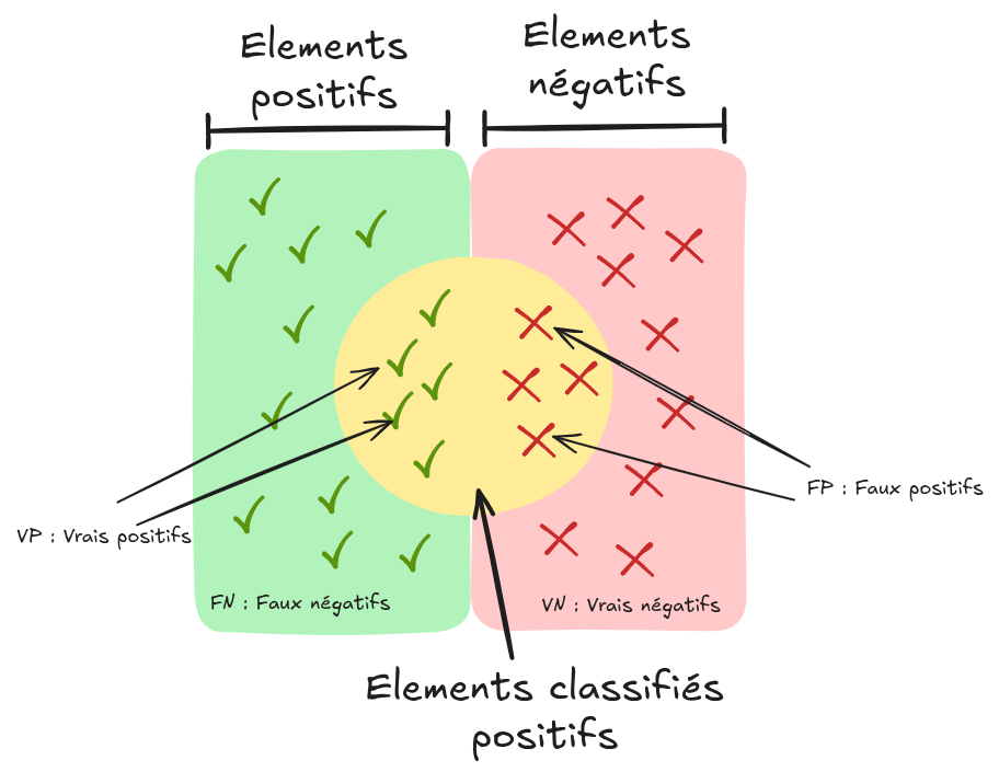
In binary classification, you can visualize the model’s predictions as follows:
 Source: Wikipedia
Here are the basic terms:
False positive (fp): An element classified as positive when it is actually negative.
True positive (vp): An element classified as positive and actually positive.
False negative (fn): An element classified as negative when it is actually positive.
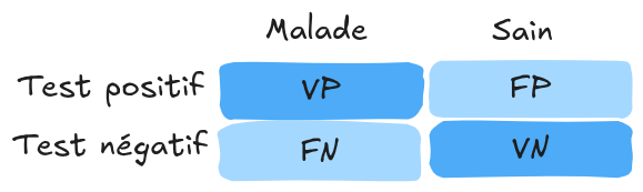
True negative (vn): An element classified as negative and actually negative. These concepts can be represented in a confusion matrix:
 Note: For multi-class classification, the confusion matrix helps identify confusions between classes.
Precision, Recall, and Specificity#
From the confusion matrix, you can calculate several metrics:
Precision: \(Precision=\frac{vp}{vp+fp}\). Proportion of positive elements correctly classified among all those classified as positive.
Recall (or sensitivity): \(Recall=\frac{vp}{vp+fn}\). Proportion of positive elements correctly classified among all positive elements.
Specificity (or selectivity): \(Specificity=\frac{vn}{vn+fp}\). Proportion of negative elements correctly classified among all negative elements.
Accuracy#
Accuracy (note: do not confuse with precision) measures the number of correct predictions out of the total predictions. Its formula is: \(Accuracy=\frac{vp+vn}{vp+vn+fp+fn}\) Note: Use with caution in case of class imbalance.
F1-Score#
The F1-score is a commonly used metric. It is the harmonic mean between precision and recall: \(F1=2 \times \frac{precision \times recall}{precision + recall}\) If precision and recall are close, the F1-score is close to their average.
ROC Curve#
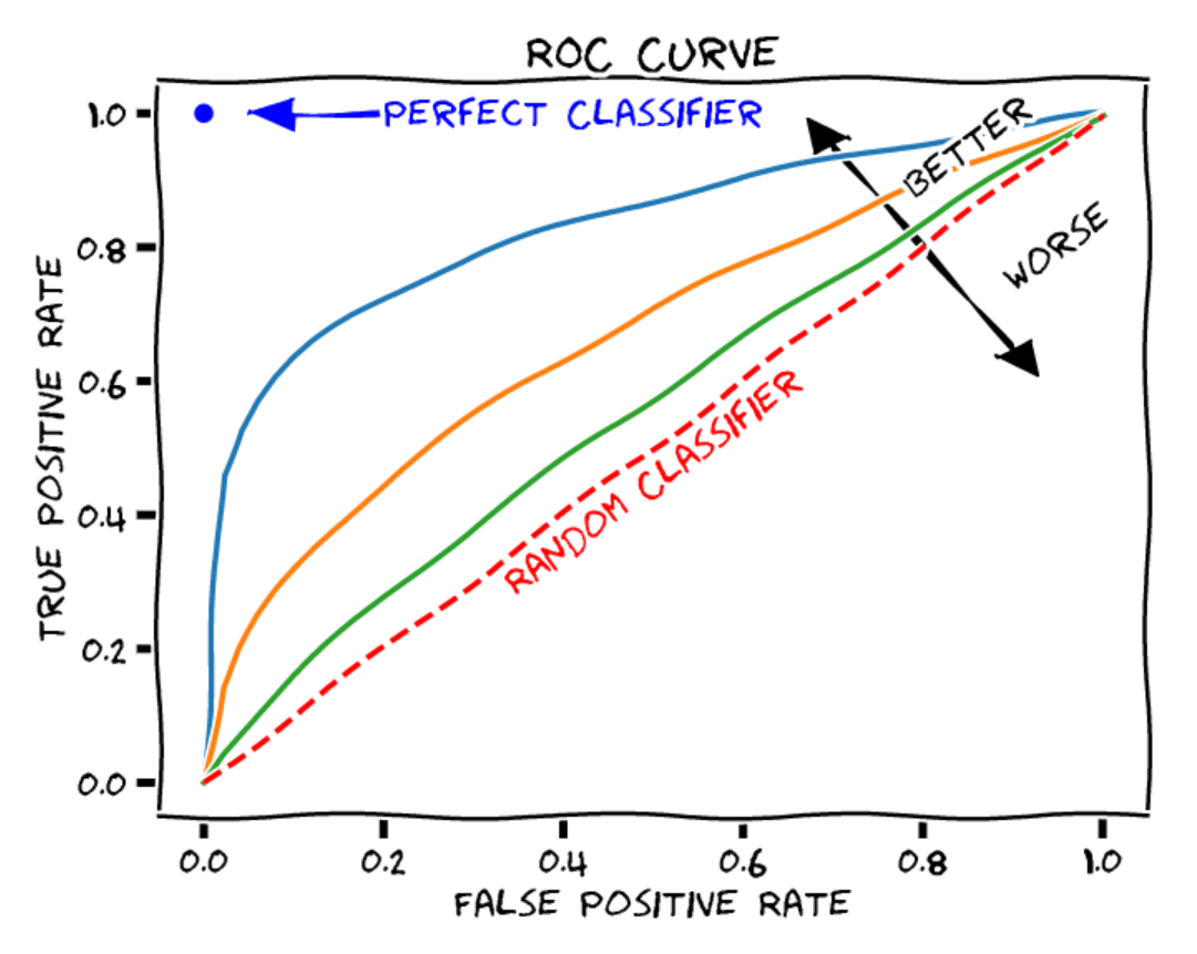
The ROC (Receiver Operating Characteristic) curve shows the performance of a binary classification model at different thresholds. It includes:
X-axis: False positive rate (\(1-specificity\)). Proportion of negative elements incorrectly classified as positive.
Y-axis: True positive rate (\(recall\)). Proportion of positive elements correctly classified. Each point on the curve corresponds to a different decision threshold.
 Source: Blogpost
To evaluate a model, calculate the area under the curve (AUROC):
Source: Blogpost
To evaluate a model, calculate the area under the curve (AUROC):Random classifier: AUROC = 0.5
Perfect classifier: AUROC = 1
Log Loss#
You can simply use the loss value on the test data as a metric. Since the loss reflects the objective, this can be sufficient in many cases.
Metrics for Regression and Autoencoders#
Mean Absolute Error (MAE)#
For regression models or autoencoders, predictions are compared to actual values by calculating a distance. The MAE (Mean Absolute Error) is the average of absolute errors: \(\text{MAE} = \frac{1}{n} \sum_{i=1}^{n} \left| y_i - \hat{y}_i \right|\)
Mean Squared Error (MSE)#
The MSE (Mean Squared Error) is often used, which is the average of the squared errors: \(\text{MSE} = \frac{1}{n} \sum_{i=1}^{n} \left( y_i - \hat{y}_i \right)^2\)
Metrics for Detection and Segmentation#
AP and mAP#
In detection, you cannot just evaluate precision. You need to consider different recall thresholds for a relevant evaluation. The average precision (AP) is calculated as follows: \(\text{AP} = \int_{0}^{1} \text{Precision}(r) \, \text{d}r\) Or discretely: \(\text{AP} = \sum_{k=1}^{K} \text{Precision}(r_k) \cdot (r_k - r_{k-1})\) Where:
\(\text{Precision}(r)\): Precision at recall \(r\)
\(K\): Number of recall evaluation points
\(r_k\) and \(r_{k-1}\): Recall at points \(k\) and \(k-1\)
The mean average precision (mAP) is the average of AP for all classes in a multi-class detection problem. It provides an overall evaluation of the model considering all classes. \(\text{mAP} = \frac{1}{C} \sum_{c=1}^{C} \text{AP}_c\)
Intersection Over Union (IoU)#
In detection and segmentation, IoU (Intersection Over Union) is a key metric. In detection, an IoU threshold is set below which a detection is considered invalid (not counted for mAP). In segmentation, IoU directly evaluates quality. \(\text{IoU} = \frac{|\text{Intersection}|}{|\text{Union}|} = \frac{|\text{Prediction} \cap \text{Ground Truth}|}{|\text{Prediction} \cup \text{Ground Truth}|}\) Note: IoU penalizes small objects and rare classes. To reduce this bias, you can use the dice coefficient.
Dice Coefficient#
In segmentation, the dice coefficient is often used instead of IoU. Its formula is: \(\text{Dice} = \frac{2 \times |\text{Prediction} \cap \text{Ground Truth}|}{|\text{Prediction}| + |\text{Ground Truth}|}\) The dice coefficient emphasizes the intersection between prediction and ground truth, giving more weight to common elements.
Evaluating Language Models#
Evaluating language models is complex. While you can use the test loss, it does not provide a precise idea of real performance. Several methods and benchmarks exist to evaluate these models based on different criteria. Sources:
Evaluating Image Generation Models#
Evaluating image generation models is complex. Human evaluation is often needed to judge the quality of generated images. Source: Blogpost on evaluating generative models