Application on a color image dataset#
import torchvision
import torch
import torch.nn as nn
import torch.nn.functional as F
import torchvision.transforms as transforms
import matplotlib.pyplot as plt
import numpy as np
Introduction to the CIFAR-10 dataset#
In this application, we will use the CIFAR-10 dataset. It contains 60,000 color images of size \(3 \times 32 \times 32\), divided into 10 classes. The classes are: airplane, automobile, bird, cat, deer, dog, frog, horse, ship, and truck. We will load the dataset using torchvision:
classes = ('plane', 'car', 'bird', 'cat','deer', 'dog', 'frog', 'horse', 'ship', 'truck')
# Transformation des données, normalisation et transformation en tensor pytorch
transform = transforms.Compose([transforms.ToTensor(),transforms.Normalize((0.5, 0.5, 0.5), (0.5, 0.5, 0.5))])

# Téléchargement et chargement du dataset
dataset = torchvision.datasets.CIFAR10(root='./../data', train=True,download=True, transform=transform)
testdataset = torchvision.datasets.CIFAR10(root='./../data', train=False,download=True, transform=transform)
print("taille d'une image : ",dataset[0][0].shape)

#Création des dataloaders pour le train, validation et test
train_dataset, val_dataset=torch.utils.data.random_split(dataset, [0.8,0.2])
train_loader = torch.utils.data.DataLoader(train_dataset, batch_size=16,shuffle=True, num_workers=2)
val_loader= torch.utils.data.DataLoader(val_dataset, batch_size=16,shuffle=True, num_workers=2)
test_loader = torch.utils.data.DataLoader(testdataset, batch_size=16,shuffle=False, num_workers=2)
Files already downloaded and verified
Files already downloaded and verified
taille d'une image :  torch.Size([3, 32, 32])
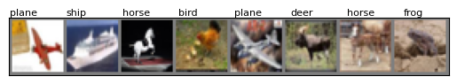
You can visualize the images and their classes:
def imshow_with_labels(img, labels):
  img = img / 2 + 0.5  # Dénormaliser
  npimg = img.numpy()
  plt.imshow(np.transpose(npimg, (1, 2, 0)))
  plt.xticks([])  # Supprimer les graduations sur l'axe des x
  plt.yticks([])  # Supprimer les graduations sur l'axe des y
  for i in range(len(labels)):
    plt.text(i * 35, -2, classes[labels[i]], color='black', fontsize=8, ha='left')

# Récupération d'un batch d'images
images, labels = next(iter(train_loader))

# Affichage des images avec leurs classes
imshow_with_labels(torchvision.utils.make_grid(images[:8]), labels[:8])
plt.show()
Designing a Convolutional Network for this Problem#
In the convolution course, we learned about the stride parameter, which represents the convolution step. With a stride of 2, the image resolution is halved at the end of the operation (provided the padding compensates for the filter size). Thus, the pooling operation can be replaced by increasing the stride. The output of a convolution layer with a stride of 1 followed by a pooling layer is the same dimension as that of a convolution layer with a stride of 2 without pooling. In this application, we will replace the pooling layers by increasing the stride of the convolutions. For more information, refer to the blog post or the article.
class cnn(nn.Module):
  def __init__(self, *args, **kwargs) -> None:
    super().__init__(*args, **kwargs)
    self.conv1=nn.Conv2d(3,8,kernel_size=3,stride=2,padding=1)
    self.conv2=nn.Conv2d(8,16,kernel_size=3,stride=2,padding=1)
    self.conv3=nn.Conv2d(16,32,kernel_size=3,stride=2,padding=1)
    self.fc=nn.Linear(4*4*32,10)

  def forward(self,x):
    x=F.relu(self.conv1(x))
    x=F.relu(self.conv2(x))
    x=F.relu(self.conv3(x))
    x=x.view(-1,4*4*32)
    output=self.fc(x)
    return output
model = cnn() # Couches d'entrée de taille 2, deux couches cachées de 16 neurones et un neurone de sortie
print(model)
print("Nombre de paramètres", sum(p.numel() for p in model.parameters()))
cnn(
  (conv1): Conv2d(3, 8, kernel_size=(3, 3), stride=(2, 2), padding=(1, 1))
  (conv2): Conv2d(8, 16, kernel_size=(3, 3), stride=(2, 2), padding=(1, 1))
  (conv3): Conv2d(16, 32, kernel_size=(3, 3), stride=(2, 2), padding=(1, 1))
  (fc): Linear(in_features=512, out_features=10, bias=True)
)
Nombre de paramètres 11162
Training the Model#
criterion = nn.CrossEntropyLoss()
epochs=5
learning_rate=0.001
optimizer=torch.optim.Adam(model.parameters(),lr=learning_rate)
for i in range(epochs):
  loss_train=0
  for images, labels in train_loader:
    preds=model(images)
    loss=criterion(preds,labels)
    optimizer.zero_grad()
    loss.backward()
    optimizer.step()
    loss_train+=loss
  if i % 1 == 0:
    print(f"step {i} train loss {loss_train/len(train_loader)}")
  loss_val=0
  for images, labels in val_loader:
    with torch.no_grad(): # permet de ne pas calculer les gradients
      preds=model(images)
      loss=criterion(preds,labels)
      loss_val+=loss
  if i % 1 == 0:
    print(f"step {i} val loss {loss_val/len(val_loader)}")
step 0 train loss 1.5988761186599731
step 0 val loss 1.4532517194747925
step 1 train loss 1.3778905868530273
step 1 val loss 1.3579093217849731
step 2 train loss 1.2898519039154053
step 2 val loss 1.2919617891311646
step 3 train loss 1.2295998334884644
step 3 val loss 1.256637692451477
step 4 train loss 1.186734914779663
step 4 val loss 1.240902304649353
You can now check the accuracy on the test data:
correct = 0
total = 0
for images,labels in test_loader:
  with torch.no_grad():
    preds=model(images)

    _, predicted = torch.max(preds.data, 1)
    total += labels.size(0)
    correct += (predicted == labels).sum().item()
test_acc = 100 * correct / total
print("Précision du modèle en phase de test : ",test_acc)
Précision du modèle en phase de test : 55.92
Using a GPU#
If you have a GPU on your computer or access to a cloud service with GPU, you can speed up the training and inference of your model. Here’s how to do it with PyTorch:
model = cnn().to('cuda') # Ajouter le .to('cuda') pour charger le modèle sur GPU
criterion = nn.CrossEntropyLoss()
epochs=5
learning_rate=0.001
optimizer=torch.optim.Adam(model.parameters(),lr=learning_rate)
for i in range(epochs):
  loss_train=0
  for images, labels in train_loader:
    images=images.to('cuda') # Ajouter le .to('cuda') pour charger les images sur GPU
    labels=labels.to('cuda') # Ajouter le .to('cuda') pour charger les labels sur GPU
    preds=model(images)
    loss=criterion(preds,labels)
    optimizer.zero_grad()
    loss.backward()
    optimizer.step()
    loss_train+=loss
  if i % 1 == 0:
    print(f"step {i} train loss {loss_train/len(train_loader)}")
  loss_val=0
  for images, labels in val_loader:
    with torch.no_grad():
      images=images.to('cuda')
      labels=labels.to('cuda')
      preds=model(images)
      loss=criterion(preds,labels)
      loss_val+=loss
  if i % 1 == 0:
    print(f"step {i} val loss {loss_val/len(val_loader)}")
/home/aquilae/anaconda3/envs/dev/lib/python3.11/site-packages/torch/autograd/graph.py:744: UserWarning: Plan failed with a cudnnException: CUDNN_BACKEND_EXECUTION_PLAN_DESCRIPTOR: cudnnFinalize Descriptor Failed cudnn_status: CUDNN_STATUS_NOT_SUPPORTED (Triggered internally at ../aten/src/ATen/native/cudnn/Conv_v8.cpp:919.)
  return Variable._execution_engine.run_backward(  # Calls into the C++ engine to run the backward pass
step 0 train loss 1.6380540132522583
step 0 val loss 1.4465171098709106
step 1 train loss 1.369913101196289
step 1 val loss 1.3735681772232056
step 2 train loss 1.2817057371139526
step 2 val loss 1.2942956686019897
step 3 train loss 1.2238909006118774
step 3 val loss 1.2601954936981201
step 4 train loss 1.186323881149292
step 4 val loss 1.2583365440368652
correct = 0
total = 0
for images,labels in test_loader:
  images=images.to('cuda')
  labels=labels.to('cuda')
  with torch.no_grad():
    preds=model(images)

    _, predicted = torch.max(preds.data, 1)
    total += labels.size(0)
    correct += (predicted == labels).sum().item()
test_acc = 100 * correct / total
print("Précision du modèle en phase de test : ",test_acc)
Précision du modèle en phase de test : 55.76
Depending on your GPU, you have likely noticed an increase in the model’s training and inference speed. This speed difference is even more pronounced with powerful GPUs and deep, parallelizable models.
Practical Exercise#
To practice, try improving the model’s performance on the CIFAR-10 dataset. You can:
Increase the number of layers
Change the number of filters per layer
Add dropout
Use batch normalization
Increase the number of epochs
Modify the learning rate Aim to achieve at least 70% accuracy.