Transfer Learning with PyTorch

To illustrate the benefits of transfer learning, we will use a small dataset containing images of ants and bees. The goal is to train a model to classify whether the insect in the image is an ant or a bee. This code is inspired by the PyTorch fine-tuning example. You can download the dataset by clicking on this link.

import torch
import torch.nn as nn
import torch.optim as optim
import numpy as np
import torchvision
from torchvision import datasets, models, transforms
import matplotlib.pyplot as plt
import os

device = torch.device("cuda:0" if torch.cuda.is_available() else "cpu")

Dataset

Let’s start by loading our dataset:

# Transformation des données
transforms = transforms.Compose([
        transforms.Resize(256),
        transforms.CenterCrop(224),
        transforms.ToTensor(),
        transforms.Normalize([0.485, 0.456, 0.406], [0.229, 0.224, 0.225]) # moyenne et ecart type utilisé pour le pre-entrainement
    ])

# Chemin vers les données
data_dir = '../data/hymenoptera_data' 

train_data = datasets.ImageFolder(os.path.join(data_dir, 'train'), transforms)
val_data= datasets.ImageFolder(os.path.join(data_dir, 'val'), transforms)

train_loader = torch.utils.data.DataLoader(train_data, batch_size=4,shuffle=True, num_workers=4)
val_loader = torch.utils.data.DataLoader(val_data, batch_size=4,shuffle=True, num_workers=4)


class_names = train_data.classes
print("Classes du dataset : ",class_names)

print("Nombre d'images d'entrainement : ",len(train_data))
print("Nombre d'images de validation : ",len(val_data))

Classes du dataset :  ['ants', 'bees']
Nombre d'images d'entrainement :  244
Nombre d'images de validation :  153

As you can see, we have very few images. We can visualize some elements of our dataset:

def imshow(inp, title=None):
    inp = inp.numpy().transpose((1, 2, 0))
    mean = np.array([0.485, 0.456, 0.406])
    std = np.array([0.229, 0.224, 0.225])
    inp = std * inp + mean
    inp = np.clip(inp, 0, 1)
    plt.imshow(inp)
    plt.title(title)

inputs, classes = next(iter(train_loader))

out = torchvision.utils.make_grid(inputs)

imshow(out, title=[class_names[x] for x in classes])

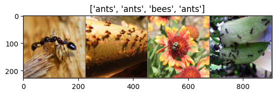
The dataset seems quite complex, as sometimes the insects occupy a very small part of the image.

Model Creation

For the model, we use the ResNet18 architecture, which is lightweight and highly effective for classification problems.

class modified_resnet18(nn.Module):
  def __init__(self,weights=None,out_class=2):
    super(modified_resnet18, self).__init__()
    # On charge le modèle pré-entrainé. Si weights=None, on charge le modèle sans les poids pré-entrainés
    self.resnet18 = models.resnet18(weights=weights) 
    # On remplace la dernière couche du modèle pour correspondre au nombre de classes de notre problème
    self.resnet18.fc = nn.Linear(512, out_class)
  
  def forward(self,x):
    return self.resnet18(x)

Training without Transfer Learning

First, we will try to train our model from scratch.

model = modified_resnet18(weights=None,out_class=len(class_names)) #weights=None pour charger le modèle sans les poids pré-entrainés
model = model.to(device)

lr=0.001
epochs=10

criterion = nn.CrossEntropyLoss()
optimizer_ft = optim.SGD(model.parameters(), lr=lr)

for epoch in range(epochs):
  loss_train=0
  for inputs, labels in train_loader:
    inputs, labels = inputs.to(device), labels.to(device)
    optimizer_ft.zero_grad()
    outputs = model(inputs)
    loss = criterion(outputs, labels)
    loss.backward()
    optimizer_ft.step()
    loss_train+=loss.item()
  
  
  model.eval()
  with torch.no_grad():
    loss_val=0
    for inputs, labels in val_loader:
      inputs, labels = inputs.to(device), labels.to(device)
      outputs = model(inputs)
      loss = criterion(outputs, labels)
      loss_val+=loss.item()
    print(f"Epoch {epoch+1}/{epochs} : train loss : {loss_train/len(train_loader)} val loss : {loss_val/len(val_loader)}")

Epoch 1/10 : train loss : 0.7068140135436761 val loss : 0.6533934359367077
Epoch 2/10 : train loss : 0.7156724578044453 val loss : 0.7215747200907805
Epoch 3/10 : train loss : 0.6751646028190362 val loss : 0.6428722785069392
Epoch 4/10 : train loss : 0.5965930917223946 val loss : 0.7239674238058237
Epoch 5/10 : train loss : 0.6105695530527928 val loss : 0.5773208579764917
Epoch 6/10 : train loss : 0.5515003006477825 val loss : 0.8412383454732406
Epoch 7/10 : train loss : 0.5839061943478272 val loss : 0.6010858137638141
Epoch 8/10 : train loss : 0.5389361244733216 val loss : 0.6349012469634031
Epoch 9/10 : train loss : 0.5367097518727427 val loss : 0.5850474796234033
Epoch 10/10 : train loss : 0.5234740852821068 val loss : 0.782087844151717

We calculate the accuracy on our validation data:

correct = 0
total = 0
with torch.no_grad():
    for inputs, labels in val_loader:
        inputs, labels = inputs.to(device), labels.to(device)
        outputs = model(inputs)
        _, predicted = torch.max(outputs, 1)
        total += labels.size(0)
        correct += (predicted == labels).sum().item()
print('Précision sur les images de validation: %d %%' % (100 * correct / total))

Précision sur les images de validation: 58 %

The accuracy is really poor (with a random model, it would be 50%)…

def visualize_model(model, num_images=6):
    model.eval()
    images_so_far = 0
    with torch.no_grad():
        for i, (inputs, labels) in enumerate(val_loader):
            inputs = inputs.to(device)
            labels = labels.to(device)
            outputs = model(inputs)
            _, preds = torch.max(outputs, 1)
            
            for j in range(inputs.size()[0]):
                images_so_far += 1
                ax = plt.subplot(num_images//2, 2, images_so_far)
                ax.axis('off')
                ax.set_title(f'predicted: {class_names[preds[j]]}')
                imshow(inputs.cpu().data[j], title=f'predicted: {class_names[preds[j]]}')

                if images_so_far == num_images:
                    return
visualize_model(model)

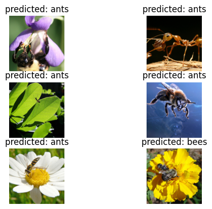
We see that the model is making random guesses. This is not surprising, as we have very few images. To train a performant model from scratch, we would need many more images, especially for a deep model.

Training with Transfer Learning

Now let’s see what we can achieve using transfer learning. The only thing that changes from the previous code is the weights parameter of our model (and hopefully, the results too).

model = modified_resnet18(weights='IMAGENET1K_V1',out_class=len(class_names)) #On charge les poids pré-entrainés sur ImageNet
model = model.to(device)

lr=0.001
epochs=10

criterion = nn.CrossEntropyLoss()
optimizer_ft = optim.SGD(model.parameters(), lr=lr)

for epoch in range(epochs):
  loss_train=0
  for inputs, labels in train_loader:
    inputs, labels = inputs.to(device), labels.to(device)
    optimizer_ft.zero_grad()
    outputs = model(inputs)
    loss = criterion(outputs, labels)
    loss.backward()
    optimizer_ft.step()
    loss_train+=loss.item()
  
  
  model.eval()
  with torch.no_grad():
    loss_val=0
    for inputs, labels in val_loader:
      inputs, labels = inputs.to(device), labels.to(device)
      outputs = model(inputs)
      loss = criterion(outputs, labels)
      loss_val+=loss.item()
    print(f"Epoch {epoch+1}/{epochs} : train loss : {loss_train/len(train_loader)} val loss : {loss_val/len(val_loader)}")

Epoch 1/10 : train loss : 0.6442642182600303 val loss : 0.5642786813087952
Epoch 2/10 : train loss : 0.30489559746423706 val loss : 0.26585672435183555
Epoch 3/10 : train loss : 0.10015173801831657 val loss : 0.22248221815635377
Epoch 4/10 : train loss : 0.03893961609325937 val loss : 0.23963456177481043
Epoch 5/10 : train loss : 0.017503870887773446 val loss : 0.21813779352352214
Epoch 6/10 : train loss : 0.011329375068107467 val loss : 0.24817544420903476
Epoch 7/10 : train loss : 0.008011038282496824 val loss : 0.22638171303939694
Epoch 8/10 : train loss : 0.005813347443854284 val loss : 0.2239722229714971
Epoch 9/10 : train loss : 0.004845750937047491 val loss : 0.23538081515699816
Epoch 10/10 : train loss : 0.003927258039885735 val loss : 0.24088036894728504

Let’s calculate the accuracy on our validation data:

correct = 0
total = 0
with torch.no_grad():
    for inputs, labels in val_loader:
        inputs, labels = inputs.to(device), labels.to(device)
        outputs = model(inputs)
        _, predicted = torch.max(outputs, 1)
        total += labels.size(0)
        correct += (predicted == labels).sum().item()
print('Précision sur les images de validation: %d %%' % (100 * correct / total))

Précision sur les images de validation: 91 %

The result is completely different. We went from 58% accuracy to 91% thanks to the use of pre-trained weights.

visualize_model(model)

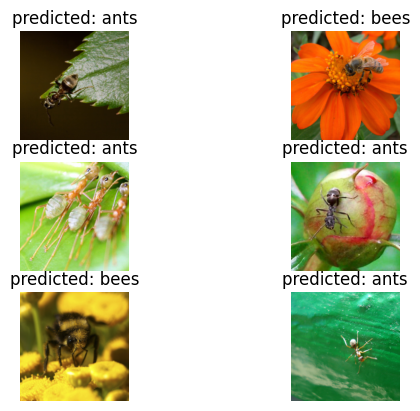
That’s much better! I hope this course has convinced you of the power of transfer learning!