Batch Normalization

Batch Normalization (or batch normalization) was introduced in 2015 in the paper Batch Normalization: Accelerating Deep Network Training by Reducing Internal Covariate Shift. It had a major impact in the field of Deep Learning. Today, normalization is almost systematically used, whether it is BatchNorm, LayerNorm, or GroupNorm (and others).

The idea behind BatchNorm is simple and related to the previous notebook. We aim to obtain preactivations following a Gaussian distribution at each layer of the network. We saw that good initialization allows this behavior, but it is not always easy, especially with many different layers.

BatchNorm normalizes the preactivations with respect to the batch dimension before passing them into the activation functions. This ensures a Gaussian distribution at each step.

This normalization does not affect optimization as it is a differentiable function.

Implementation

Code Review

We will review the code from the previous notebook to implement batch normalization.

import torch
import torch.nn.functional as F
%matplotlib inline

words = open('../05_NLP/prenoms.txt', 'r').read().splitlines()
chars = sorted(list(set(''.join(words))))
stoi = {s:i+1 for i,s in enumerate(chars)}
stoi['.'] = 0
itos = {i:s for s,i in stoi.items()}

block_size = 3 # Contexte

def build_dataset(words):  
  X, Y = [], []
  
  for w in words:
    context = [0] * block_size
    for ch in w + '.':
      ix = stoi[ch]
      X.append(context)
      Y.append(ix)
      context = context[1:] + [ix] 

  X = torch.tensor(X)
  Y = torch.tensor(Y)
  print(X.shape, Y.shape)
  return X, Y

import random
random.seed(42)
random.shuffle(words)
n1 = int(0.8*len(words))
n2 = int(0.9*len(words))

Xtr,  Ytr  = build_dataset(words[:n1])     # 80%
Xdev, Ydev = build_dataset(words[n1:n2])   # 10%
Xte,  Yte  = build_dataset(words[n2:])     # 10%

torch.Size([180834, 3]) torch.Size([180834])
torch.Size([22852, 3]) torch.Size([22852])
torch.Size([22639, 3]) torch.Size([22639])

embed_dim=10 # Dimension de l'embedding de C
hidden_dim=200 # Dimension de la couche cachée

C = torch.randn((46, embed_dim))
W1 = torch.randn((block_size*embed_dim, hidden_dim))*0.01 # On initialise les poids à une petite valeur
b1 = torch.randn(hidden_dim) *0 # On initialise les biais à 0
W2 = torch.randn((hidden_dim, 46))*0.01
b2 = torch.randn(46)*0 
parameters = [C, W1, b1, W2, b2]
for p in parameters:
  p.requires_grad = True

Here is our forward propagation code:

batch_size = 32

ix = torch.randint(0, Xtr.shape[0], (batch_size,))
  
# Forward
Xb, Yb = Xtr[ix], Ytr[ix] 
emb = C[Xb] 
embcat = emb.view(emb.shape[0], -1)
hpreact = embcat @ W1 + b1 

h = torch.tanh(hpreact) 
logits = h @ W2 + b2 
loss = F.cross_entropy(logits, Yb)

Implementing BatchNorm

According to the article, here is the information:

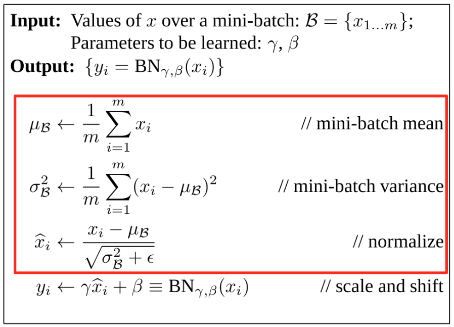
First, we need to normalize.

To do this, we calculate the mean and standard deviation of hpreact and then normalize using these values:

epsilon=1e-6
hpreact_mean = hpreact.mean(dim=0, keepdim=True)
hpreact_std= hpreact.std(dim=0, keepdim=True)
hpreact_norm = (hpreact - hpreact_mean) / (hpreact_std+epsilon)

We can now integrate this normalization into the forward propagation.

C = torch.randn((46, embed_dim))
W1 = torch.randn((block_size*embed_dim, hidden_dim))*0.01 # On initialise les poids à une petite valeur
b1 = torch.randn(hidden_dim) *0 # On initialise les biais à 0
W2 = torch.randn((hidden_dim, 46))*0.01
b2 = torch.randn(46)*0 
# Paramètres de batch normalization
bngain = torch.ones((1, hidden_dim))
bnbias = torch.zeros((1, hidden_dim))

parameters = [C, W1, b1, W2, b2, bngain, bnbias]
for p in parameters:
  p.requires_grad = True

And in forward propagation, we will have:

batch_size = 32

ix = torch.randint(0, Xtr.shape[0], (batch_size,))
  
# Forward
Xb, Yb = Xtr[ix], Ytr[ix] 
emb = C[Xb] 
embcat = emb.view(emb.shape[0], -1)
hpreact = embcat @ W1 + b1 

# Batch normalization
bnmean = hpreact.mean(0, keepdim=True)
bnstd = hpreact.std(0, keepdim=True)
hpreact = bngain * (hpreact - bnmean) / bnstd + bnbias

h = torch.tanh(hpreact) 
logits = h @ W2 + b2 
loss = F.cross_entropy(logits, Yb)

The Problem with Batch Normalization

Upon reflection, we can identify potential issues related to BatchNorm:

An example is affected by other elements in the batch: Normalizing along the batch dimension means that the values of each example within the batch are influenced by other examples. This might seem problematic, but in practice, it’s actually a good thing. Using random batches at each epoch provides regularization, reducing the risk of overfitting the data. However, if you want to avoid this issue, you can use other normalization methods that do not normalize along the batch dimension. In practice, BatchNorm is still widely used because it works very well empirically.

Testing on a single element: During training, each element is influenced by other elements in its batch. However, during inference, when using the model on a single element, we can no longer apply BatchNorm. This is a problem because we want to avoid different behavior during training and inference.

To solve this problem, we have two solutions:

• We can calculate the mean and variance over all elements at the end of training and use these values. In practice, we don’t want to perform an additional iteration over the entire dataset just for this, so no one does it this way.

• Another solution is to update the mean and variance throughout training using an EMA (exponential moving average). At the end of training, we will have a good approximation of the mean and variance of all training elements.

In practice, we can implement it like this in Python:

C = torch.randn((46, embed_dim))
W1 = torch.randn((block_size*embed_dim, hidden_dim))*0.01 # On initialise les poids à une petite valeur
b1 = torch.randn(hidden_dim) *0 # On initialise les biais à 0
W2 = torch.randn((hidden_dim, 46))*0.01
b2 = torch.randn(46)*0 
# Paramètres de batch normalization
bngain = torch.ones((1, hidden_dim))
bnbias = torch.zeros((1, hidden_dim))
bnmean_running = torch.zeros((1, hidden_dim))
bnstd_running = torch.ones((1, hidden_dim))

parameters = [C, W1, b1, W2, b2, bngain, bnbias]
for p in parameters:
  p.requires_grad = True

batch_size = 32

ix = torch.randint(0, Xtr.shape[0], (batch_size,))
  
# Forward
Xb, Yb = Xtr[ix], Ytr[ix] 
emb = C[Xb] 
embcat = emb.view(emb.shape[0], -1)
hpreact = embcat @ W1 + b1 

# Batch normalization
bnmeani = hpreact.mean(0, keepdim=True)
bnstdi = hpreact.std(0, keepdim=True)
hpreact = bngain * (hpreact - bnmeani) / bnstdi + bnbias
with torch.no_grad(): # On ne veut pas calculer de gradient pour ces opérations
    bnmean_running = 0.999 * bnmean_running + 0.001 * bnmeani
    bnstd_running = 0.999 * bnstd_running + 0.001 * bnstdi

h = torch.tanh(hpreact) 
logits = h @ W2 + b2 
loss = F.cross_entropy(logits, Yb)

Note: In our implementation, we chose 0.001 for our EMA. In the BatchNorm layer of PyTorch, this parameter is defined by momentum and its default value is 0.1. In practice, the choice of this value depends on the size of the batch relative to the size of the training dataset. For a large batch with a small dataset, you can take 0.1, for example. For a small batch with a large dataset, we prefer a smaller value.

Let’s now test the training of our model to verify that the layer works. For this small model, we won’t see a difference in performance.

lossi = []
max_steps = 200000

for i in range(max_steps):
  ix = torch.randint(0, Xtr.shape[0], (batch_size,))
  Xb, Yb = Xtr[ix], Ytr[ix] 
  emb = C[Xb] 
  embcat = emb.view(emb.shape[0], -1)
  hpreact = embcat @ W1 + b1 
  
  # Batch normalization
  bnmeani = hpreact.mean(0, keepdim=True)
  bnstdi = hpreact.std(0, keepdim=True)
  hpreact = bngain * (hpreact - bnmeani) / bnstdi + bnbias
  with torch.no_grad(): # On ne veut pas calculer de gradient pour ces opérations
      bnmean_running = 0.999 * bnmean_running + 0.001 * bnmeani
      bnstd_running = 0.999 * bnstd_running + 0.001 * bnstdi
    
  h = torch.tanh(hpreact) 
  logits = h @ W2 + b2 
  loss = F.cross_entropy(logits, Yb)
  
  for p in parameters:
    p.grad = None
  loss.backward()
  lr = 0.1 if i < 100000 else 0.01 
  for p in parameters:
    p.data += -lr * p.grad
  if i % 10000 == 0:
    print(f'{i:7d}/{max_steps:7d}: {loss.item():.4f}')
  lossi.append(loss.log10().item())

      0/ 200000: 3.8241
  10000/ 200000: 1.9756
  20000/ 200000: 2.7151
  30000/ 200000: 2.3287
  40000/ 200000: 2.1411
  50000/ 200000: 2.3207
  60000/ 200000: 2.3250
  70000/ 200000: 2.0320
  80000/ 200000: 2.0615
  90000/ 200000: 2.2468
 100000/ 200000: 2.2081
 110000/ 200000: 2.1418
 120000/ 200000: 1.9665
 130000/ 200000: 1.8572
 140000/ 200000: 2.0577
 150000/ 200000: 2.1804
 160000/ 200000: 1.8604
 170000/ 200000: 1.9810
 180000/ 200000: 1.8228
 190000/ 200000: 1.9977

Additional Considerations

Bias: Batch norm normalizes the preactivations of the weights. This normalization cancels out the bias (since it shifts the distribution, while we recentre it). When using BatchNorm, we can do without the bias. In practice, if you leave a bias, it’s not a problem, but it’s a network parameter that will be unnecessary.

Placement of BatchNorm: Based on what we’ve seen, it makes sense to place BatchNorm before the activation function. In practice, some prefer to place it after the activation layer, so don’t be surprised if you encounter this in the literature or in code.

Other Normalizations

We will quickly review other normalizations used for training neural networks.

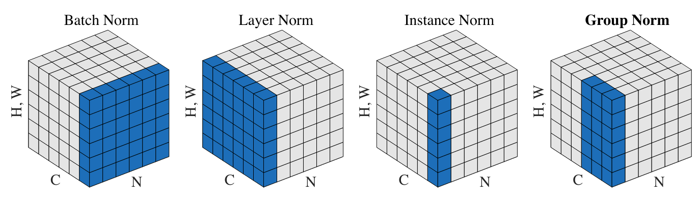
Figure extracted from the article

Layer Normalization: This normalization layer is also very frequently used, especially in language models (GPT, Llama). It involves normalizing across all activations of the layer rather than along the batch axis. In our implementation, this would simply mean changing:

# Batch normalization
bnmeani = hpreact.mean(0, keepdim=True)  
bnstdi = hpreact.std(0, keepdim=True)   
# Layer normalization
bnmeani = hpreact.mean(1, keepdim=True)  
bnstdi = hpreact.std(1, keepdim=True)  

Instance Normalization: This layer normalizes activations on each channel of each element independently.

Group Normalization: This layer is a kind of fusion between LayerNorm and InstanceNorm, as normalization is calculated on groups of channels (if the size of a group is 1, it’s InstanceNorm and if the size of a group is C, it’s LayerNorm)