Variational Autoencoders#
In this course, we introduce variational autoencoders, also known as variational autoencoders (VAE). We start with a quick recap of Course 4 on Autoencoders, then we introduce the use of VAEs as generative models. This course is inspired by a blog post and does not delve into the mathematical details of how VAEs work. The figures used in this notebook also come from the blog post.
Recap on Autoencoders#
An autoencoder is a neural network shaped like an hourglass. It consists of an encoder that encodes information into a reduced-dimensional latent space and a decoder that reconstructs the original data from the latent representation.
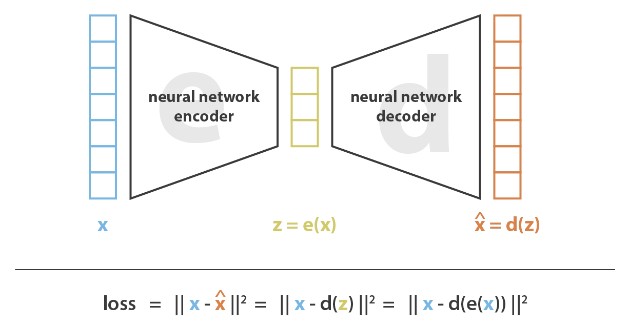
Autoencoders can be used for many things, but their primary role is data compression. It is a compression method that uses gradient descent optimization.
Intuition#
Imagine that the latent space of our decoder is regular (represented by a known probability distribution). In this case, we could sample a random element from this distribution to generate new data. In practice, in a classic autoencoder, the latent representation is not regular, making it impossible to use for generating data. Thinking about it, this makes sense. The loss function of the autoencoder is based solely on the quality of the reconstruction and imposes no constraints on the shape of the latent space. Therefore, we would like to impose the shape of the latent space of our autoencoder to generate new data from this latent space.
Variational Autoencoder#
A variational autoencoder (VAE) is an autoencoder constrained to have a latent space that allows data generation. It has regulated training for this purpose. The idea is to encode our input into a data distribution instead of a single value (as in an AE). In practice, our encoder will predict two values representing a normal distribution: the mean \(\mu\) and the variance \(\sigma^2\). The VAE works as follows during training:
The encoder encodes the input into a probability distribution by predicting \(\mu\) and \(\sigma^2\).
A value is sampled from the Gaussian distribution described by \(\mu\) and \(\sigma^2\).
The decoder reconstructs the data from the sampled value.
Backpropagation is applied to update the weights.
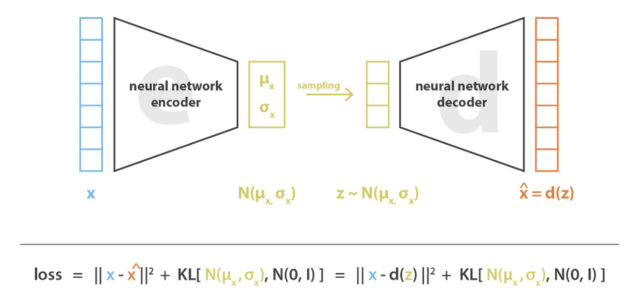
To ensure that the training does what we want, we need to add a term to the loss function: the Kullback-Leibler divergence. This term helps push the distribution to be a standard normal distribution.
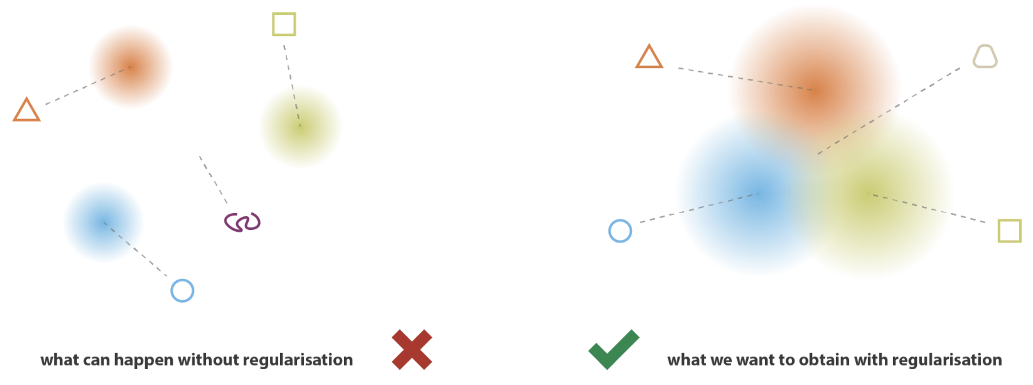
For consistent data generation, there are two things to consider:
Continuity: Points close in the latent space will produce close data in the output space.
Completeness: Decoded points must make sense in the output space.
The Kullback-Leibler divergence ensures these two properties. If we only used the reconstruction loss, the VAE could behave like an AE by predicting almost zero variances (which would be almost equivalent to a point, as predicted by an AE’s encoder).
The Kullback-Leibler divergence encourages the distributions in the latent space to be close to each other. This allows for consistent data generation when sampling.
 Note: There is an important theoretical aspect behind Variational Autoencoders, but we will not delve into the details in this course. To learn more, you can refer to Stanford’s CS236 course and in particular this link.