Convolutional Networks with PyTorch#
Importing Required Libraries#
import torch
import torch.nn as nn
import torch.nn.functional as F
import torchvision.transforms as T
from torchvision import datasets
from torch.utils.data import DataLoader
import matplotlib.pyplot as plt
Classification on MNIST#
To demonstrate the effectiveness of 2D convolutional neural networks, we’ll start with the classic example of classifying digits from 0 to 9 in the MNIST dataset. We’ll use the code from previous notebooks, particularly the one on fully connected networks.
Retrieving the Dataset and Creating Data Loaders for Training#
transform=T.ToTensor() # Pour convertir les éléments en tensor torch directement
dataset = datasets.MNIST(root='./../data', train=True, download=True,transform=transform)
test_dataset = datasets.MNIST(root='./../data', train=False,transform=transform)
plt.imshow(dataset[1][0].permute(1,2,0).numpy(), cmap='gray')
plt.show()
print("Le chiffre sur l'image est un "+str(dataset[1][1]))
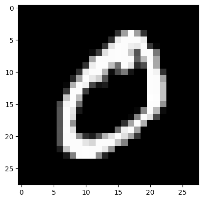
Le chiffre sur l'image est un 0
train_dataset, validation_dataset=torch.utils.data.random_split(dataset, [0.8,0.2])
train_loader = DataLoader(train_dataset, batch_size=64, shuffle=True)
val_loader= DataLoader(validation_dataset, batch_size=64, shuffle=True)
test_loader = DataLoader(test_dataset, batch_size=64, shuffle=False)
Creating a Convolutional Neural Network in PyTorch#
class cnn(nn.Module):
  def __init__(self, *args, **kwargs) -> None:
    super().__init__(*args, **kwargs)
    self.conv1=nn.Conv2d(1,8,kernel_size=3,padding=1) # Couche de convolution de 8 filtres
    self.conv2=nn.Conv2d(8,16,kernel_size=3,padding=1) # Couche de convolution de 16 filtres
    self.conv3=nn.Conv2d(16,32,kernel_size=3,padding=1) # Couche de convolution de 32 filtres
    self.pool1=nn.MaxPool2d((2,2)) # Couche de max pooling
    self.pool2=nn.MaxPool2d((2,2))
    self.fc=nn.Linear(32*7*7,10)

  # La fonction forward est la fonction appelée lorsqu'on fait model(x)
  def forward(self,x):
    x=F.relu(self.conv1(x))
    x=self.pool1(x)
    x=F.relu(self.conv2(x))
    x=self.pool2(x)
    x=F.relu(self.conv3(x))
    x=x.view(-1,32*7*7) # Pour convertir la feature map de taille 32x7x7 en taille vecteur de taille 1568
    output=self.fc(x)
    return output
model = cnn()
print(model)
print("Nombre de paramètres", sum(p.numel() for p in model.parameters()))
cnn(
  (conv1): Conv2d(1, 8, kernel_size=(3, 3), stride=(1, 1), padding=(1, 1))
  (conv2): Conv2d(8, 16, kernel_size=(3, 3), stride=(1, 1), padding=(1, 1))
  (conv3): Conv2d(16, 32, kernel_size=(3, 3), stride=(1, 1), padding=(1, 1))
  (pool1): MaxPool2d(kernel_size=(2, 2), stride=(2, 2), padding=0, dilation=1, ceil_mode=False)
  (pool2): MaxPool2d(kernel_size=(2, 2), stride=(2, 2), padding=0, dilation=1, ceil_mode=False)
  (fc): Linear(in_features=1568, out_features=10, bias=True)
)
Nombre de paramètres 21578
As you can see, the number of parameters in this model is much lower than in a classic fully connected network.
Training the Model#
Let’s define the loss function and training hyperparameters:
criterion = nn.CrossEntropyLoss()
epochs=5
learning_rate=0.001
optimizer=torch.optim.Adam(model.parameters(),lr=learning_rate)
Now, let’s train the model:
for i in range(epochs):
  loss_train=0
  for images, labels in train_loader:
    preds=model(images)
    loss=criterion(preds,labels)
    optimizer.zero_grad()
    loss.backward()
    optimizer.step()
    loss_train+=loss
  if i % 1 == 0:
    print(f"step {i} train loss {loss_train/len(train_loader)}")
  loss_val=0
  for images, labels in val_loader:
    with torch.no_grad(): # permet de ne pas calculer les gradients
      preds=model(images)
      loss=criterion(preds,labels)
      loss_val+=loss
  if i % 1 == 0:
    print(f"step {i} val loss {loss_val/len(val_loader)}")
step 0 train loss 0.318773478269577
step 0 val loss 0.08984239399433136
step 1 train loss 0.08383051306009293
step 1 val loss 0.0710655003786087
step 2 train loss 0.05604167655110359
step 2 val loss 0.0528845489025116
step 3 train loss 0.04518255963921547
step 3 val loss 0.051780227571725845
step 4 train loss 0.03614392504096031
step 4 val loss 0.0416230633854866
And let’s calculate the accuracy on the test set:
correct = 0
total = 0
for images,labels in test_loader:
  with torch.no_grad():
    preds=model(images)

    _, predicted = torch.max(preds.data, 1)
    total += labels.size(0)
    correct += (predicted == labels).sum().item()
test_acc = 100 * correct / total
print("Précision du modèle en phase de test : ",test_acc)
Précision du modèle en phase de test : 98.64
As you can see, we achieve an accuracy of approximately 99%, compared to 97.5% with a fully connected network that has 10 times more parameters.
Softmax and Result Interpretation#
If we run the model on an element, we get a vector like this:
images,labels=next(iter(test_loader))

#Isolons un élément
image,label=images[0].unsqueeze(0),labels[0].unsqueeze(0) # Le unsqueeze permet de garder la dimension batch
pred=model(image)
print(pred)
tensor([[ -9.6179,  -5.1802,  -2.6094,   0.9121, -16.0603,  -8.6510, -30.0099,
          14.4031,  -9.0074,  -2.0431]], grad_fn=<AddmmBackward0>)
Upon closely examining the results, we see that the value of the 7th element is the highest. Therefore, the model predicted a 3. Let’s verify with our label:
print(label)
tensor([7])
It is indeed a 7. However, we would prefer to have a probability of class membership. This is more readable and provides an easily interpretable confidence level.
For this, we use the softmax activation function.
This function is defined as follows: \(\sigma(z)_i = \frac{e^{z_i}}{\sum_{j=1}^{K} e^{z_j}}\) where \(K\) is the number of classes in the model.
This function is called softmax because it amplifies the maximum value while reducing the others. We use it to obtain a probability distribution, as the sum of the values for the \(K\) classes equals 1.
print(F.softmax(pred))
tensor([[3.6964e-11, 3.1266e-09, 4.0884e-08, 1.3833e-06, 5.8867e-14, 9.7215e-11,
         5.1481e-20, 1.0000e+00, 6.8068e-11, 7.2027e-08]],
       grad_fn=<SoftmaxBackward0>)
/tmp/ipykernel_232253/3904022211.py:1: UserWarning: Implicit dimension choice for softmax has been deprecated. Change the call to include dim=X as an argument.
  print(F.softmax(pred))
The values are now probabilities, and we see that the 7 is predicted with a 99.9% probability. Therefore, the model is quite confident in its prediction.
Other Applications#
Convolutional networks have proven to be particularly interesting in the field of image processing. They are also used in audio and video processing, for example.
The following notebooks in this course show applications of convolutional networks on more interesting cases than MNIST. It is recommended to have a GPU or use the notebooks on Google Colab for reasonable training times (you can still follow the course without training the model).