Diffusion Models#
In this course, we introduce diffusion models, also known as diffusion models. These models were introduced in 2020 in the paper Denoising Diffusion Probabilistic Models. Since then, they have been widely used for image generation, and very effectively. They are powerful and easy to guide, but they have a major drawback: they are very slow. This course is inspired by the CVPR 2022 Tutorial and the blogpost. The figures used in this notebook come from these two sources.
How Does It Work?#
Diffusion models work in two main steps: adding noise (diffusion process) and removing noise (reverse process or denoising process). Both steps are iterative, meaning noise is added and removed gradually.
First Step: The Diffusion Process#
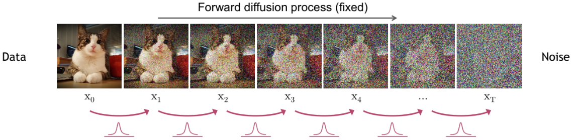
The first step of a diffusion model involves taking an image from a dataset. This dataset is represented by a complex probability distribution. The diffusion process iteratively adds Gaussian noise to the image to gradually reduce its complexity until a simple Gaussian distribution is obtained.
The following figure shows the diffusion process:
 You can see how the distribution evolves (becoming less and less complex):
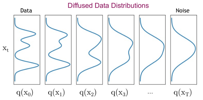 The diffusion process progressively destroys the structure of the input image.
The diffusion process occurs in multiple steps called diffusion steps. At each step, a predetermined amount of Gaussian noise is added to the image. The more steps there are, the less noise is added each time. In practice, the more steps there are, the more stable the model becomes and the higher the quality of the generated images, but this increases computation time. Often, a large number of steps is chosen (1000 in the original paper).
Second Step: The Reverse Process#
But what is the point of adding noise to an image?
In fact, the diffusion process generates training data for the reverse process.
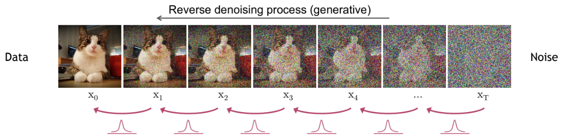
The idea of the reverse process is to learn how to go from the Gaussian distribution (obtained through diffusion) back to the original images. We want to recover the image from the Gaussian noise of the last step of the diffusion process. Thus, we can also generate new images from a sample of the Gaussian distribution.
Note: There is some similarity with normalizing flows or variational autoencoders.
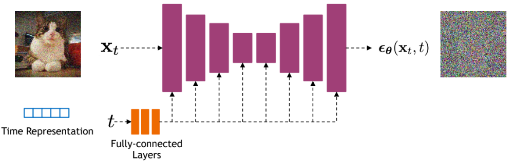
 For each denoising step, a neural network is used that takes as input the image at step \(t\) and the diffusion step \(t\) and aims to predict the Gaussian noise (\(\mu\) and \(\sigma^2\)) added to the image during the step \(t-1 \Rightarrow t\).
Note: Predicting the noise actually allows us to predict the image at step \(t-1\).
Note 2: The same network is used at each step; there is not a different network for each diffusion step.
For each denoising step, a neural network is used that takes as input the image at step \(t\) and the diffusion step \(t\) and aims to predict the Gaussian noise (\(\mu\) and \(\sigma^2\)) added to the image during the step \(t-1 \Rightarrow t\).
Note: Predicting the noise actually allows us to predict the image at step \(t-1\).
Note 2: The same network is used at each step; there is not a different network for each diffusion step.
The model used is generally a U-Net. To learn more about the U-Net architecture, you can refer to Course 3 on Convolutional Networks. In practice, for very powerful models (like Stable Diffusion), a variant of the U-Net incorporating the transformer architecture is used.
Are Diffusion Models Hierarchical VAEs?#
As mentioned earlier, diffusion models can be seen as VAEs or normalizing flows. Let’s look at the possible analogy with a VAE, and more specifically a hierarchical VAE. A hierarchical VAE is a VAE with multiple steps of image generation (decoder). For our diffusion model, the diffusion process would correspond to the encoder of the VAE, while the reverse process would correspond to the multiple hierarchical steps of the VAE. In practice, there are a few notable differences:
The encoder is fixed (non-trainable) for the diffusion model; it is simply the addition of noise.
The latent space has the same dimension as the input image (which is not the case for a VAE).
The model used for diffusion is the same at each diffusion step. For a hierarchical VAE, a different model is used at each step. The same kind of analogy can be made with a normalizing flow. I invite you to consult the CVPR 2022 Tutorial to learn more.
Main Problem with Diffusion Models#
As explained earlier, the diffusion and denoising processes benefit from a large number of steps. Each denoising step requires a forward pass of the U-Net network. If there are 1000 diffusion steps, the network must be called 1000 times to generate a single image.
The problem with diffusion models is immediately apparent: they are very, very slow.
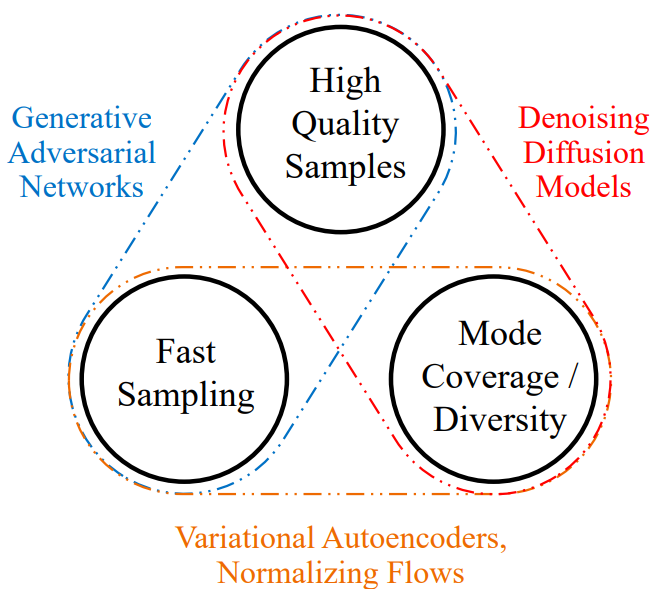 Figure extracted from the article.
Diffusion models are much more powerful than GANs, VAEs, and normalizing flows for image generation. Therefore, these are the models we would like to use first. It is therefore necessary to find methods to accelerate these diffusion models through various techniques. This course does not detail the existing techniques to accelerate these models, but the CVPR 2022 Tutorial covers the subject very well (even though new techniques have been introduced since then). For information, high-quality images can now be generated in about ten steps (compared to 1000 before).
Diffusion models are a major research topic right now, and there are still many problems to solve. Here are a few of them:
Why are diffusion models so much more effective than VAEs and normalizing flows? Should we redirect research efforts to these alternatives now that we have learned a lot about diffusion?
Is it possible to reduce the process to a single step to generate images?
Can the diffusion architecture help with discriminative applications?
Is the U-Net architecture really the best choice for diffusion?
Can diffusion models be applied to other types of data (such as text, for example)?