My First Neural Network#
In this course, we will build our first neural network using the micrograd library. Micrograd is a simple and easy-to-understand library specialized in automatic gradient calculation. To master it better, you can watch the introduction video by Andrej Karpathy (in English). This notebook is also inspired by the notebook provided in the micrograd repository.
Building a Neural Network with micrograd#
#!pip install micrograd # uncomment to install micrograd
import random
import numpy as np
import matplotlib.pyplot as plt
from micrograd.engine import Value
from micrograd.nn import Neuron, Layer, MLP
# Pour la reproducibilité
np.random.seed(1337)
random.seed(1337)
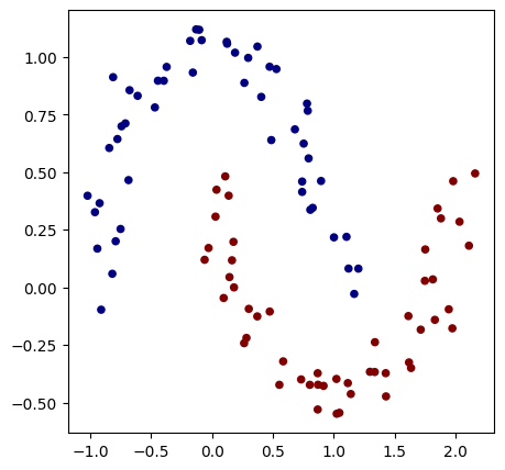
To build a neural network, we first need a problem to solve. We use the make_moons function from scikit-learn, which generates a dataset. To simplify the loss calculation in the following steps, we replace the classes 0 and 1 with -1 and 1.
Dataset Initialization#
from sklearn.datasets import make_moons, make_blobs
X, y = make_moons(n_samples=100, noise=0.1) # 100 éléments et un bruit Gaussien d'écart type 0.1 ajouté sur les données

print("Les données d'entrée sont de la forme : ",X[1])

y = y*2 - 1 # Pour avoir y=-1 ou y=1 (au lieu de 0 et 1)

# Visualisation des données en 2D
plt.figure(figsize=(5,5))
plt.scatter(X[:,0], X[:,1], c=y, s=20, cmap='jet')
Les données d'entrée sont de la forme : [-0.81882941 0.05879006]
<matplotlib.collections.PathCollection at 0x177253e50>
Creating the Neural Network#
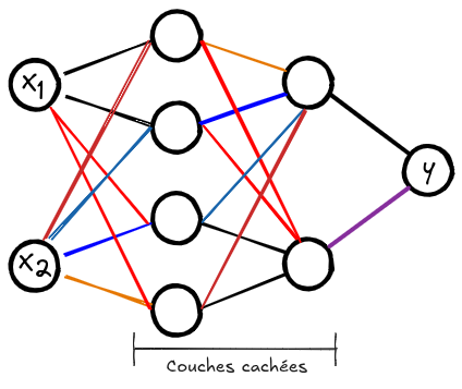
Now, we will initialize our neural network. It takes 2 values as input and must produce a label of -1 or 1.
The network we will build has 2 hidden layers, each containing 16 neurons. Each neuron acts as a logistic regression, making our network a non-linear combination of multiple logistic regressions.
Here is an overview of the architecture of this network:
# Initialisation du modèle
model = MLP(2, [16, 16, 1]) # Couches d'entrée de taille 2, deux couches cachées de 16 neurones et un neurone de sortie
print(model)
print("Nombre de paramètres", len(model.parameters()))
MLP of [Layer of [ReLUNeuron(2), ReLUNeuron(2), ReLUNeuron(2), ReLUNeuron(2), ReLUNeuron(2), ReLUNeuron(2), ReLUNeuron(2), ReLUNeuron(2), ReLUNeuron(2), ReLUNeuron(2), ReLUNeuron(2), ReLUNeuron(2), ReLUNeuron(2), ReLUNeuron(2), ReLUNeuron(2), ReLUNeuron(2)], Layer of [ReLUNeuron(16), ReLUNeuron(16), ReLUNeuron(16), ReLUNeuron(16), ReLUNeuron(16), ReLUNeuron(16), ReLUNeuron(16), ReLUNeuron(16), ReLUNeuron(16), ReLUNeuron(16), ReLUNeuron(16), ReLUNeuron(16), ReLUNeuron(16), ReLUNeuron(16), ReLUNeuron(16), ReLUNeuron(16)], Layer of [LinearNeuron(16)]]
Nombre de paramètres 337
Stochastic Gradient Descent (SGD)#
Before continuing, let’s review stochastic gradient descent (SGD). To apply the gradient descent algorithm on a dataset of size \(N\), in theory, you would need to calculate the loss and gradient for each element before updating the weights. This method ensures a decrease in loss at each iteration, but it is very costly for datasets where \(N\) is large (often \(N>10⁶\)). Additionally, you would need to store the gradients of all \(N\) elements in memory, which is impossible for large datasets. To solve this problem, we use mini-batches, which are groups of samples from the dataset. Optimization is done as in classical gradient descent, but the weights are updated at each mini-batch (thus more frequently). This makes the optimization process faster and allows handling large amounts of data. The size of a mini-batch is called batch size and is often 16, 32, or 64. To learn more about stochastic gradient descent, check Wikipedia or this blogpost. Let’s define a Python function to retrieve batch_size random elements from our dataset.
def get_batch(batch_size=64):
  ri = np.random.permutation(X.shape[0])[:batch_size]
  Xb, labels = X[ri], y[ri]
  #inputs = [list(map(Value, xrow)) for xrow in Xb] # OLD
  # Conversion des inputs en Value pour pouvoir utiliser micrograd
  inputs = [list([Value(xrow[0]),Value(xrow[1])]) for xrow in Xb]
  return inputs,labels
Loss Function#
To train our neural network, we need to define a loss function. In our case, we have two classes and we want to maximize the margin between examples belonging to different classes. Unlike the negative log-likelihood loss used previously, we aim to maximize this margin, making our method more robust to new elements. We use the max-margin loss, defined by: \(\text{loss} = \max(0, 1 - y_i \cdot \text{score}_i)\)
def loss_function(scores,labels):
  # La fonction .relu() prend le maximum entre 0 et la valeur de 1 - yi*scorei
  losses = [(1 - yi*scorei).relu() for yi, scorei in zip(labels, scores)]
  # On divise le loss par le nombre d'éléments du mini-batch
  data_loss = sum(losses) * (1.0 / len(losses))
  return data_loss
Model Training#
Now that we have the key elements for training, it’s time to define our training loop
# Définissons nos hyper-paramètres d'entraînement
batch_size=128
iteration=50
We can now start training our model:
for k in range(iteration):

  # On récupère notre mini-batch random
  inputs,labels=get_batch(batch_size=batch_size)

  # On fait appel au modèle pour calculer les scores Y
  scores = list(map(model, inputs))

  # On calcule le loss
  loss=loss_function(scores,labels)


  accuracy = [(label > 0) == (scorei.data > 0) for label, scorei in zip(labels, scores)]
  accuracy=sum(accuracy) / len(accuracy)

  # Remise à zéro de valeurs de gradients avant de les calculer
  model.zero_grad()
  # Calcul des gradients grâce à l'autograd de micrograd
  loss.backward()

  # Mise à jour des poids avec les gradients calculés (SGD)
  learning_rate = 1.0 - 0.9*k/100 # On diminue le learning rate au fur et à mesure de l'entraînement
  for p in model.parameters():
      p.data -= learning_rate * p.grad

  if k % 1 == 0:
      print(f"step {k} loss {loss.data}, accuracy {accuracy*100}%")
step 0 loss 0.8862514464368221, accuracy 50.0%
step 1 loss 1.7136790633950052, accuracy 81.0%
step 2 loss 0.733396126728699, accuracy 77.0%
step 3 loss 0.7615247055858604, accuracy 82.0%
step 4 loss 0.35978083334534205, accuracy 84.0%
step 5 loss 0.3039360355411295, accuracy 86.0%
step 6 loss 0.2716587340549048, accuracy 89.0%
step 7 loss 0.25896576803013205, accuracy 91.0%
step 8 loss 0.2468445503533517, accuracy 91.0%
step 9 loss 0.26038987927745966, accuracy 91.0%
step 10 loss 0.23569710047306525, accuracy 91.0%
step 11 loss 0.2403768930229477, accuracy 92.0%
step 12 loss 0.20603128479123115, accuracy 91.0%
step 13 loss 0.22061157796029193, accuracy 93.0%
step 14 loss 0.19010711228374735, accuracy 92.0%
step 15 loss 0.21687609382796402, accuracy 93.0%
step 16 loss 0.18642445342175254, accuracy 92.0%
step 17 loss 0.2064478196088666, accuracy 92.0%
step 18 loss 0.15299793102189654, accuracy 94.0%
step 19 loss 0.18164592701596197, accuracy 93.0%
step 20 loss 0.15209012673698674, accuracy 92.0%
step 21 loss 0.17985784886850317, accuracy 93.0%
step 22 loss 0.13186703020683818, accuracy 95.0%
step 23 loss 0.13971668862318976, accuracy 95.0%
step 24 loss 0.1052987732627048, accuracy 96.0%
step 25 loss 0.11575214222251122, accuracy 95.0%
step 26 loss 0.10138692709798285, accuracy 97.0%
step 27 loss 0.13983249990522056, accuracy 95.0%
step 28 loss 0.13439433831552547, accuracy 92.0%
step 29 loss 0.14946491199753797, accuracy 95.0%
step 30 loss 0.08058651087395295, accuracy 97.0%
step 31 loss 0.08894402478347964, accuracy 97.0%
step 32 loss 0.14846171628770516, accuracy 95.0%
step 33 loss 0.08534324122933533, accuracy 97.0%
step 34 loss 0.06930425973662234, accuracy 97.0%
step 35 loss 0.10224309625633382, accuracy 95.0%
step 36 loss 0.05690038135075194, accuracy 97.0%
step 37 loss 0.04361190103707672, accuracy 97.0%
step 38 loss 0.04085954349889362, accuracy 98.0%
step 39 loss 0.06115860793647568, accuracy 97.0%
step 40 loss 0.06712605274368717, accuracy 99.0%
step 41 loss 0.1007776535938798, accuracy 95.0%
step 42 loss 0.047219615684323896, accuracy 97.0%
step 43 loss 0.03229533112572595, accuracy 99.0%
step 44 loss 0.028346610758982437, accuracy 99.0%
step 45 loss 0.05011775341000794, accuracy 99.0%
step 46 loss 0.09321634150737651, accuracy 96.0%
step 47 loss 0.055859575569553566, accuracy 98.0%
step 48 loss 0.02709965160774589, accuracy 99.0%
step 49 loss 0.054945465674614925, accuracy 98.0%
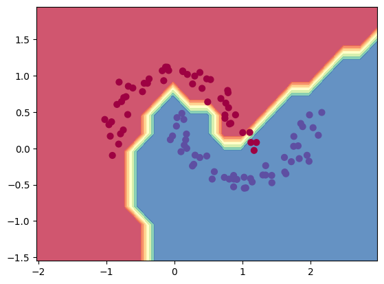
As you can see, the loss does not consistently decrease at each training step. This is due to stochastic gradient descent: not considering the entire dataset at each iteration introduces randomness. However, the loss decreases on average during training, allowing us to obtain a robust model more quickly.
# Visualisation de la frontière de décision
h = 0.25
x_min, x_max = X[:, 0].min() - 1, X[:, 0].max() + 1
y_min, y_max = X[:, 1].min() - 1, X[:, 1].max() + 1
xx, yy = np.meshgrid(np.arange(x_min, x_max, h),
                     np.arange(y_min, y_max, h))
Xmesh = np.c_[xx.ravel(), yy.ravel()]
inputs = [list(map(Value, xrow)) for xrow in Xmesh]
scores = list(map(model, inputs))
Z = np.array([s.data > 0 for s in scores])
Z = Z.reshape(xx.shape)

fig = plt.figure()
plt.contourf(xx, yy, Z, cmap=plt.cm.Spectral, alpha=0.8)
plt.scatter(X[:, 0], X[:, 1], c=y, s=40, cmap=plt.cm.Spectral)
plt.xlim(xx.min(), xx.max())
plt.ylim(yy.min(), yy.max())
(-1.548639298268643, 1.951360701731357)