Implementing a VAE

In this notebook, we will implement a VAE to generate images from the MNIST dataset. We start with a classic autoencoder to show that such an architecture does not allow generating new elements.

import numpy as np
import random
import torch
import torch.nn as nn
import torch.nn.functional as F
import torchvision.transforms as T
from torchvision import datasets
from torch.utils.data import DataLoader
import matplotlib.pyplot as plt

/home/aquilae/anaconda3/envs/dev/lib/python3.11/site-packages/tqdm/auto.py:21: TqdmWarning: IProgress not found. Please update jupyter and ipywidgets. See https://ipywidgets.readthedocs.io/en/stable/user_install.html
  from .autonotebook import tqdm as notebook_tqdm

Dataset

We start by loading the MNIST dataset:

transform = T.Compose([
    T.ToTensor(),
    T.Normalize((0.5,), (0.5,))
])
dataset = datasets.MNIST(root='./../data', train=True, download=True,transform=transform)
test_dataset = datasets.MNIST(root='./../data', train=False,transform=transform)

print("taille du dataset d'entrainement : ",len(dataset))
print("taille d'une image : ",dataset[0][0].numpy().shape) 

train_dataset, validation_dataset=torch.utils.data.random_split(dataset, [0.8,0.2])
train_loader = DataLoader(train_dataset, batch_size=64, shuffle=True)
val_loader= DataLoader(validation_dataset, batch_size=64, shuffle=True)
test_loader = DataLoader(test_dataset, batch_size=64, shuffle=False)

taille du dataset d'entrainement :  60000
taille d'une image :  (1, 28, 28)

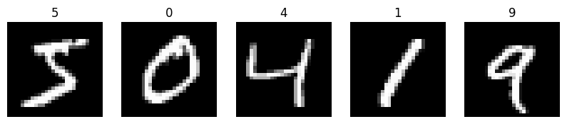
# Visualisons quelques images
plt.figure(figsize=(10, 10))
for i in range(5):
  plt.subplot(1, 5, i+1)
  plt.imshow(dataset[i][0].squeeze(), cmap='gray')
  plt.axis('off')
  plt.title(dataset[i][1])

Autoencoder on MNIST

We build the architecture of our autoencoder:

class AE(nn.Module):
    def __init__(self):
        super(AE, self).__init__()
        self.encoder = nn.Sequential(
            nn.Conv2d(1, 16, 3, stride=2, padding=1),  # -> [16, 14, 14]
            nn.ReLU(),
            nn.Conv2d(16, 8, 3, stride=2, padding=1),  # -> [8, 7, 7]
            nn.ReLU(),
            nn.Conv2d(8, 8, 3, stride=2, padding=1)   # -> [8, 4, 4]
        )
        self.decoder = nn.Sequential(
            nn.ConvTranspose2d(8, 8, 3, stride=2, padding=1, output_padding=0),
            nn.ReLU(),
            nn.ConvTranspose2d(8, 16, 3, stride=2, padding=1, output_padding=1),
            nn.ReLU(),
            nn.ConvTranspose2d(16, 1, 3, stride=2, padding=1, output_padding=1),
            nn.Tanh()
        )
    def forward(self, x):
        x = self.encoder(x)
        x = self.decoder(x)
        return x
dummy_input = torch.randn(1, 1, 28, 28) 
model = AE()
output = model(dummy_input)
print(output.shape)

torch.Size([1, 1, 28, 28])

We define our training hyperparameters:

epochs = 10
criterion = nn.MSELoss()
optimizer = torch.optim.Adam(model.parameters(), lr=0.001)

We proceed to train the model:

for epoch in range(epochs): 
    for img,_ in train_loader:
        optimizer.zero_grad()
        recon = model(img)
        loss = criterion(recon, img)
        loss.backward()
        optimizer.step()
    print('epoch [{}/{}], loss:{:.4f}'.format(epoch+1, epochs, loss.item()))

epoch [1/10], loss:0.0330
epoch [2/10], loss:0.0220
epoch [3/10], loss:0.0199
epoch [4/10], loss:0.0186
epoch [5/10], loss:0.0171
epoch [6/10], loss:0.0172
epoch [7/10], loss:0.0175
epoch [8/10], loss:0.0168
epoch [9/10], loss:0.0159
epoch [10/10], loss:0.0148

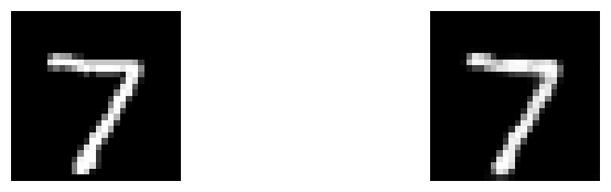
We check the model’s behavior on the test data:

for data in test_loader:
    img, _ = data
    recon = model(img)
    break
plt.figure(figsize=(9, 2))
plt.gray()
plt.subplot(1, 2, 1)
plt.imshow(img[0].detach().numpy().squeeze())
plt.axis('off')
plt.subplot(1, 2, 2)
plt.imshow(recon[0].detach().numpy().squeeze())
plt.axis('off')
plt.show()

We now visualize the latent space and the distribution of the 10 classes within this space.

# On commence par extraire les représentations latentes des données de test
latents = []
labels = []

with torch.no_grad():
    for data, target in test_loader:
        latent = model.encoder(data)
        latents.append(latent)
        labels.append(target)

latents = torch.cat(latents)
labels = torch.cat(labels)

We use the T-SNE method to extract 2D representations and visualize the data.

from sklearn.manifold import TSNE

latents_flat = latents.view(latents.size(0), -1)
tsne = TSNE(n_components=2, random_state=0)
latent_2d = tsne.fit_transform(latents_flat)

plt.figure(figsize=(10, 8))
scatter = plt.scatter(latent_2d[:, 0], latent_2d[:, 1], c=labels, cmap='viridis', alpha=0.5)
plt.colorbar(scatter)
plt.title('Visualisation de l\'espace latent de MNIST avec un autoencodeur CNN')
plt.xlabel('Dimension 1')
plt.ylabel('Dimension 2')
plt.show()

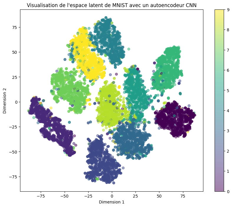
As expected, the classes are well separated in the latent space. However, there are many empty spaces, making it difficult to sample a random point in the latent space and expect to generate a coherent real data point.

We look at what we get by generating an image from a random point in the latent space.

latent_dim = (8, 4, 4)
sampled_latent = torch.randn(latent_dim).unsqueeze(0)

# On générer l'image avec le décodeur
with torch.no_grad():
    generated_image = model.decoder(sampled_latent)

generated_image = generated_image.squeeze().numpy()  # Supprimer la dimension batch et convertir en numpy
generated_image = (generated_image + 1) / 2  # Dénormaliser l'image (car Tanh est utilisé)
plt.imshow(generated_image, cmap='gray')
plt.title("Image générée")
plt.axis('off')
plt.show()

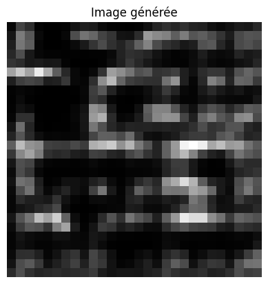
As expected, this generates nothing coherent.

Variational Autoencoder

Now, we use the same architecture (more or less) but with a VAE to see if we can generate data.

class VAE(nn.Module):
    def __init__(self,latent_dim=8):
        super(VAE, self).__init__()
        # Encodeur
        self.encoder_conv = nn.Sequential(
            nn.Conv2d(1, 16, 3, stride=2, padding=1),  # -> [16, 14, 14]
            nn.ReLU(),
            nn.Conv2d(16, 8, 3, stride=2, padding=1),  # -> [8, 7, 7]
            nn.ReLU(),
            nn.Conv2d(8, 8, 3, stride=2, padding=1)   # -> [8, 4, 4]
        )
        self.fc_mu = nn.Linear(8*4*4, latent_dim)
        self.fc_logvar = nn.Linear(8*4*4, latent_dim)
        
        # Décodeur
        self.decoder_fc = nn.Sequential(
            nn.Linear(latent_dim, 8*4*4),
            nn.ReLU()
        )
        self.decoder_conv = nn.Sequential(
            nn.ConvTranspose2d(8, 8, 3, stride=2, padding=1, output_padding=0),
            nn.ReLU(),
            nn.ConvTranspose2d(8, 16, 3, stride=2, padding=1, output_padding=1),
            nn.ReLU(),
            nn.ConvTranspose2d(16, 1, 3, stride=2, padding=1, output_padding=1),
            nn.Tanh()
        )
    
    def encode(self, x):
        h = self.encoder_conv(x)
        h = h.view(h.size(0), -1)
        mu = self.fc_mu(h)
        logvar = self.fc_logvar(h)
        return mu, logvar
    
    def reparametrize(self, mu, logvar):
        std = torch.exp(0.5 * logvar)
        eps = torch.randn_like(std)
        return mu + eps * std
    
    def decode(self, z):
        h = self.decoder_fc(z)
        h = h.view(h.size(0), 8, 4, 4)
        return self.decoder_conv(h)
    
    def forward(self, x):
        mu, logvar = self.encode(x)
        z = self.reparametrize(mu, logvar)
        return self.decode(z), mu, logvar
    
dummy_input = torch.randn(1, 1, 28, 28)
model = VAE()
output,mu,logvar = model(dummy_input)  
print(output.shape, mu.shape, logvar.shape)

torch.Size([1, 1, 28, 28]) torch.Size([1, 8]) torch.Size([1, 8])

epochs = 10
criterion = nn.MSELoss()
optimizer = torch.optim.Adam(model.parameters(), lr=0.001)

def loss_function(recon_x, x, mu, logvar):
    MSE = F.mse_loss(recon_x, x, reduction='sum')
    KLD = -0.5 * torch.sum(1 + logvar - mu.pow(2) - logvar.exp())
    return MSE + KLD

for epoch in range(epochs): 
    for data,_ in train_loader:
        optimizer.zero_grad()
        recon, mu, logvar = model(data)
        loss = loss_function(recon, data, mu, logvar)
        loss.backward()
        optimizer.step()
    print(f'Epoch {epoch}, Loss: {loss / len(train_loader.dataset)}')

Epoch 0, Loss: 0.1811039298772812
Epoch 1, Loss: 0.14575038850307465
Epoch 2, Loss: 0.14808794856071472
Epoch 3, Loss: 0.14365650713443756
Epoch 4, Loss: 0.14496898651123047
Epoch 5, Loss: 0.13169685006141663
Epoch 6, Loss: 0.1442883014678955
Epoch 7, Loss: 0.14070650935173035
Epoch 8, Loss: 0.12996357679367065
Epoch 9, Loss: 0.1352960765361786

latents = []
labels = []

with torch.no_grad():
    for data, target in test_loader:
        mu, logvar = model.encode(data)
        latents.append(mu)
        labels.append(target)

latents = torch.cat(latents)
labels = torch.cat(labels)

from sklearn.manifold import TSNE

tsne = TSNE(n_components=2, random_state=0)
latent_2d = tsne.fit_transform(latents)

import matplotlib.pyplot as plt

plt.figure(figsize=(10, 8))
scatter = plt.scatter(latent_2d[:, 0], latent_2d[:, 1], c=labels, cmap='viridis', alpha=0.5)
plt.colorbar(scatter)
plt.title('Visualisation de l\'espace latent de MNIST avec un VAE')
plt.xlabel('Dimension 1')
plt.ylabel('Dimension 2')
plt.show()

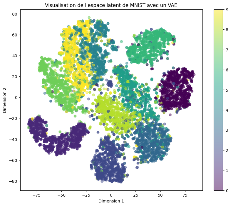
We observe that the latent space is still very scattered. This is explained by the difference between the reconstruction loss and the Kullback-Leibler divergence. In our training, the reconstruction loss was much more significant than the divergence. We can now generate images. Since the latent space does not have the desired characteristics of continuity and completeness, the generated elements may not necessarily resemble real digits.

latent_dim = 8
num_images = 10  
images_per_row = 5  

sampled_latents = torch.randn(num_images, latent_dim)

with torch.no_grad():
    generated_images = model.decode(sampled_latents)

generated_images = generated_images.squeeze().numpy()  # Supprimer la dimension batch et convertir en numpy
generated_images = (generated_images + 1) / 2  # Dénormaliser les images (car Tanh est utilisé)

fig, axes = plt.subplots(2, images_per_row, figsize=(15, 6))

for i, ax in enumerate(axes.flat):
    ax.imshow(generated_images[i], cmap='gray')
    ax.axis('off')

plt.suptitle("Images générées à partir de points échantillonnés dans l'espace latent d'un VAE")
plt.show()

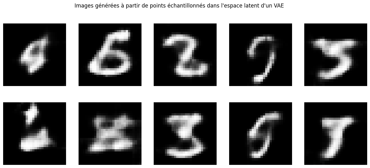
As expected, some generated images do not really make sense. As an exercise, you can try to improve the latent representation to generate coherent images every time. Note, there is always a trade-off to be made between reconstruction quality and latent space.