Autoencoder for Denoising

Intuition

What is Denoising?

Denoising involves removing unwanted noise from an image. This is a crucial task in image processing. Our goal is to input a noisy image into the network and obtain a clean image as output.

Figure extracted from article.

Using an Autoencoder for Denoising

To use the autoencoder architecture for this task, simply input a noisy image (which we generated) into the decoder, have it reconstruct the image, and compare the reconstructed image to the original, noise-free image.

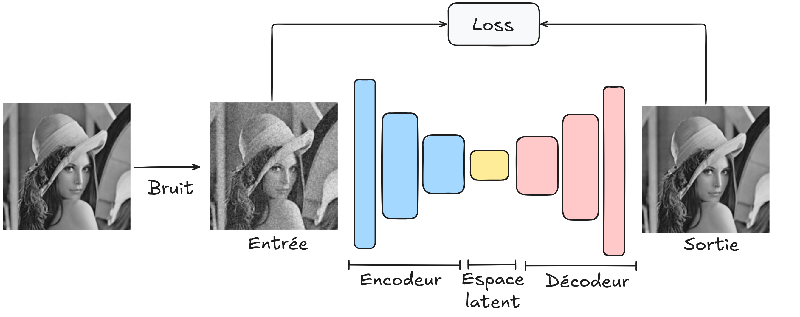
Using this architecture, we aim to create a robust denoising model capable of denoising all images. For training, a large image dataset is required, and care must be taken to ensure that the generated noise is similar to that encountered in real images.

Denoising with an Autoencoder in PyTorch

Once again, we use the MNIST dataset. We will generate artificial noise on the images and train our autoencoder to remove this noise to obtain a clean image.

import numpy as np
import torch
import torch.nn as nn
import torch.nn.functional as F
import torchvision.transforms as T
from torchvision import datasets
from torch.utils.data import DataLoader
import matplotlib.pyplot as plt

Dataset and DataLoader

transform=T.ToTensor() # Pour convertir les éléments en tensor torch directement
dataset = datasets.MNIST(root='./../data', train=True, download=True,transform=transform)
test_dataset = datasets.MNIST(root='./../data', train=False,transform=transform)
train_dataset, validation_dataset=torch.utils.data.random_split(dataset, [0.8,0.2])
train_loader = DataLoader(train_dataset, batch_size=64, shuffle=True)
val_loader= DataLoader(validation_dataset, batch_size=64, shuffle=True)
test_loader = DataLoader(test_dataset, batch_size=64, shuffle=False)

Noise Generation

Let’s apply noise to visualize how the image degrades based on the noise level.

image,_=dataset[0]
# Le paramètre dans le np.sqrt correspond à la variance désirée donc np.sqrt(...) est l'écart type
# torch.randn génére des valeurs aléatoire extraites d'une distribution gaussienne de mean 0 et variance 1
imageNoisy1 = image + np.sqrt(0.001)*torch.randn(1, 28, 28)
imageNoisy2 = image + np.sqrt(0.01)*torch.randn(1, 28, 28)
imageNoisy3 = image + np.sqrt(0.1)*torch.randn(1, 28, 28)

plt.subplot(2, 2, 1)
plt.imshow(image.squeeze().numpy(), cmap='gray')
plt.title("Image originale")

plt.subplot(2, 2, 2)
plt.imshow(imageNoisy1.squeeze().numpy(), cmap='gray')
plt.title("Faible bruit")

plt.subplot(2, 2, 3)
plt.imshow(imageNoisy2.squeeze().numpy(), cmap='gray')
plt.title("Bruit moyen")

plt.subplot(2, 2, 4)
plt.imshow(imageNoisy3.squeeze().numpy(), cmap='gray')
plt.title("Fort bruit")

plt.tight_layout()
plt.show()

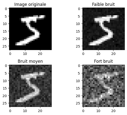
We will use a medium noise level during training. Then, we can observe how our denoising autoencoder performs on other noise levels.

Creating Our Model

For this complex task, we use a convolutional autoencoder.

# Nous réutilisons les fonctions introduites dans l'exemple de segmentation du cours 3 
def conv_relu_bn(input_channels, output_channels, kernel_size, stride, padding):
  return nn.Sequential(
    nn.Conv2d(input_channels, output_channels, kernel_size, stride, padding),
    nn.ReLU(),
    nn.BatchNorm2d(output_channels,momentum=0.01)
  )
    
def convT_relu_bn(input_channels, output_channels, kernel_size, stride, padding):
  return nn.Sequential(
    nn.ConvTranspose2d(input_channels, output_channels, kernel_size, stride, padding),
    nn.ReLU(),
    nn.BatchNorm2d(output_channels,momentum=0.01)
  )
    
    
class ae_conv(nn.Module):
  def __init__(self, *args, **kwargs) -> None:
    super().__init__(*args, **kwargs)

    self.encoder = nn.Sequential( # Sequential permet de groupe une série de transformation
      conv_relu_bn(1,8,kernel_size=3,stride=2,padding=1),
      conv_relu_bn(8,16,kernel_size=3,stride=2,padding=1),
      conv_relu_bn(16,32,kernel_size=3,stride=1,padding=1),
    )
    self.decoder = nn.Sequential(
      convT_relu_bn(32,16,kernel_size=4,stride=2,padding=1),
      convT_relu_bn(16,8,kernel_size=4,stride=2,padding=1),
      nn.Conv2d(8,1,kernel_size=3,stride=1,padding=1),
      nn.Sigmoid()
    )
  
  def forward(self,x): 
    x = self.encoder(x)
    denoise = self.decoder(x)
    return denoise

model = ae_conv() # Couches d'entrée de taille 2, deux couches cachées de 16 neurones et un neurone de sortie
print("Nombre de paramètres", sum(p.numel() for p in model.parameters()))

Nombre de paramètres 16385

Model Training

criterion = nn.MSELoss()
epochs=10
learning_rate=0.001
optimizer=torch.optim.Adam(model.parameters(),lr=learning_rate)

for i in range(epochs):
  loss_train=0
  for images, _ in train_loader:
    images=images+np.sqrt(0.01)*torch.randn(images.shape)
    recons=model(images)
    loss=criterion(recons,images)
    optimizer.zero_grad()
    loss.backward()
    optimizer.step()
    loss_train+=loss   
  if i % 1 == 0:
    print(f"step {i} train loss {loss_train/len(train_loader)}")
  loss_val=0    
  for images, _ in val_loader:
    with torch.no_grad():
      images=images+np.sqrt(0.01)*torch.randn(images.shape)
      recons=model(images)
      loss=criterion(recons,images)
      loss_val+=loss 
  if i % 1 == 0:
    print(f"step {i} val loss {loss_val/len(val_loader)}")

step 0 train loss 0.0253756046295166
step 0 val loss 0.010878251865506172
step 1 train loss 0.00976449716836214
step 1 val loss 0.008979358710348606
step 2 train loss 0.00827114749699831
step 2 val loss 0.007526080124080181
step 3 train loss 0.00706455297768116
step 3 val loss 0.0066648973152041435
step 4 train loss 0.006312613375484943
step 4 val loss 0.005955129396170378
step 5 train loss 0.00576859712600708
step 5 val loss 0.005603262223303318
step 6 train loss 0.0055686105042696
step 6 val loss 0.005487256217747927
step 7 train loss 0.0054872902110219
step 7 val loss 0.005444051697850227
step 8 train loss 0.0054359594359993935
step 8 val loss 0.005416598636657
step 9 train loss 0.005397486500442028
step 9 val loss 0.005359680857509375

images,_=next(iter(test_loader))
variance=0.01
#Isolons un élément
fig, axs = plt.subplots(2, 3, figsize=(10, 6)) 
for i in range(2):
  image=images[i].unsqueeze(0)
  noisy_image=image+np.sqrt(variance)*torch.randn(image.shape)

  with torch.no_grad():
      recons=model(noisy_image)

  # Image d'origine
  axs[i][0].imshow(noisy_image[0].squeeze().cpu().numpy(), cmap='gray')
  axs[i][0].set_title('Image d\'origine')
  axs[i][0].axis('off')

  # Image reconstruite
  axs[i][1].imshow(recons[0].squeeze().cpu().numpy(), cmap='gray')
  axs[i][1].set_title('Image reconstruite')
  axs[i][1].axis('off')

  axs[i][2].imshow(image[0].squeeze().cpu().numpy(), cmap='gray')
  axs[i][2].set_title('Image de base')
  axs[i][2].axis('off')
plt.show()

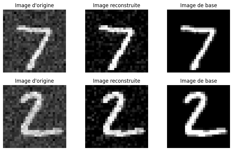
The results of our denoising are quite good, although some artifacts remain. By varying the variance parameter, you can visualize what the denoising autoencoder is capable of on other noise levels.

Exercise

You can try training the model on images with random noise levels (within certain variance values) to see if the model can generalize to any Gaussian noise within this range. You might need to make the model more complex and add more epochs during training.

U-Net: You can also try testing the U-Net architecture (see lesson 3 on segmentation) for the denoising task and compare the results with the autoencoder.