Normalizing Flow#
In this course, we introduce normalizing flows, generative models for representation learning. Less known than VAEs, GANs, or diffusion models, they still have many advantages.
GANs and VAEs cannot precisely evaluate the probability distribution. GANs do not do this at all, while VAEs use the ELBO. This causes problems during training: VAEs often generate blurry images, and GANs can fall into mode collapse.
Normalizing flows offer a solution to these issues.
How Does It Work?#
A normalizing flow is a series of bijective transformations. We use them to model complex distributions, such as those of images, by transforming them into a simple distribution, like a standard normal distribution.
To train them, we maximize the likelihood of the data. Essentially, we minimize the negative log-likelihood with respect to the actual probability density of the data. By adjusting the parameters of the transformations, we ensure that the distribution generated by the flow is as close as possible to the target distribution.
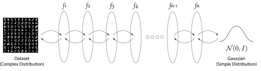
Figure from blogpost.
Advantages and Disadvantages#
Here are the main advantages of normalizing flows:
Their training is very stable
They converge more easily than GANs or VAEs
No need to generate noise to create data
However, there are also disadvantages:
They are less expressive than GANs or VAEs
The latent space is limited by the need for bijective functions and volume preservation. As a result, it is difficult to interpret because it is high-dimensional.
The generated results are often worse than those of GANs or VAEs.
Note: There is an important theoretical aspect behind normalizing flows, but we will not go into detail here. If you want to learn more, you can consult the Stanford CS236 course, specifically at this link.