数据增强#
您知道,深度学习模型的潜力受到可用训练数据量的限制。一般来说,我们需要大量的数据:最先进的视觉模型是在数十亿张图像上训练的,而 NLP 模型(如 LLM)则是在数万亿个 token 上训练的。
通常,获取高质量的标注数据是一项复杂且成本高昂的任务。
是否可以通过巧妙的变换来人工增加我们的数据?
是的!这是可行的,这种技术被称为数据增强。在本部分中,我们将探讨图像数据增强的不同方法,并简要介绍 NLP 和音频数据增强的可能性。
图像数据增强#
本部分介绍的数据增强技术已被证明对深度学习模型的训练非常有帮助。不过,需要谨慎使用,因为某些类型的数据增强可能不符合我们的训练目标(例如,如果目标是检测躺着的人,则应避免将图像旋转 90 度)。
为了介绍不同的数据增强方法,我们将使用 PyTorch,特别是其 torchvision 库,它提供了丰富的数据增强技术选择。
首先,我们从基础图像开始:
from PIL import Image
image_pil=Image.open("images/tigrou.png")
image_pil

将图像转换为 PyTorch 张量。
import torchvision.transforms as T
transform=T.Compose([T.ToTensor(),T.Resize((360,360))])
image=transform(image_pil)[0:3,:,:]
/home/aquilae/anaconda3/envs/dev/lib/python3.11/site-packages/tqdm/auto.py:21: TqdmWarning: IProgress not found. Please update jupyter and ipywidgets. See https://ipywidgets.readthedocs.io/en/stable/user_install.html
  from .autonotebook import tqdm as notebook_tqdm
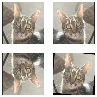
水平/垂直翻转与旋转#
数据增强的一种简单方法是对图像进行翻转(水平或垂直)或旋转。例如,倒置的猫仍然是猫。
注意:如果需要区分“猫”和“倒置的猫”这两个类别,则不应使用这种技术。必须始终明确自己的需求。
import matplotlib.pyplot as plt

horiz_flip=T.Compose([T.RandomHorizontalFlip(p=1)])
image_horiz_flip=horiz_flip(image)
vert_flip=T.Compose([T.RandomVerticalFlip(p=1)])
image_vert_flip=vert_flip(image)
rot=T.Compose([T.RandomRotation(degrees=90)])
image_rot=rot(image)

plt.figure(figsize=(5,5))
plt.subplot(221)
plt.imshow(image.permute(1,2,0))
plt.axis("off")
plt.subplot(222)
plt.imshow(image_horiz_flip.permute(1,2,0))
plt.axis("off")
plt.subplot(223)
plt.imshow(image_vert_flip.permute(1,2,0))
plt.axis("off")
plt.subplot(224)
plt.imshow(image_rot.permute(1,2,0))
plt.axis("off")
plt.show()
Clipping input data to the valid range for imshow with RGB data ([0..1] for floats or [0..255] for integers).
Clipping input data to the valid range for imshow with RGB data ([0..1] for floats or [0..255] for integers).
Clipping input data to the valid range for imshow with RGB data ([0..1] for floats or [0..255] for integers).
Clipping input data to the valid range for imshow with RGB data ([0..1] for floats or [0..255] for integers).
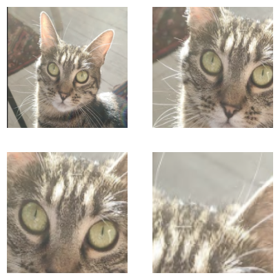
图像裁剪#
另一种技术是裁剪图像的一部分,并将裁剪后的区域作为输入图像。可选用 中心裁剪(CenterCrop)或 随机裁剪(RandomCrop)。
注意:使用这种方法时,必须确保目标对象在裁剪区域内。如果裁剪尺寸过小,或目标对象在图像中所占比例较低,这种数据增强可能会产生负面影响(见最后一张图)。
crop=T.Compose([T.RandomCrop(200)])
image_crop=crop(image)
center_crop=T.Compose([T.CenterCrop(150)])
image_center_crop=center_crop(image)

crop_small=T.Compose([T.RandomCrop(100)])
image_crop_small=crop_small(image)

plt.figure(figsize=(5,5))
plt.subplot(221)
plt.imshow(image.permute(1,2,0))
plt.axis("off")
plt.subplot(222)
plt.imshow(image_crop.permute(1,2,0))
plt.axis("off")
plt.subplot(223)
plt.imshow(image_center_crop.permute(1,2,0))
plt.axis("off")
plt.subplot(224)
plt.imshow(image_crop_small.permute(1,2,0))
plt.axis("off")
plt.show()
Clipping input data to the valid range for imshow with RGB data ([0..1] for floats or [0..255] for integers).
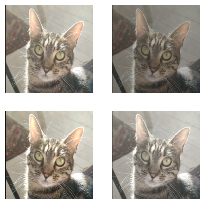
对比度、亮度、饱和度与色调#
还可以通过 ColorJitter 变换来调整图像的亮度(brightness)、对比度(contrast)、饱和度(saturation)和色调(hue)。
bright=T.Compose([T.ColorJitter(brightness=0.8)])
image_bright=bright(image)
contr=T.Compose([T.ColorJitter(contrast=0.8)])
image_contr=contr(image)

satur=T.Compose([T.ColorJitter(saturation=0.8)])
image_satur=satur(image)

plt.figure(figsize=(5,5))
plt.subplot(221)
plt.imshow(image.permute(1,2,0))
plt.axis("off")
plt.subplot(222)
plt.imshow(image_bright.permute(1,2,0))
plt.axis("off")
plt.subplot(223)
plt.imshow(image_contr.permute(1,2,0))
plt.axis("off")
plt.subplot(224)
plt.imshow(image_satur.permute(1,2,0))
plt.axis("off")
plt.show()
Clipping input data to the valid range for imshow with RGB data ([0..1] for floats or [0..255] for integers).
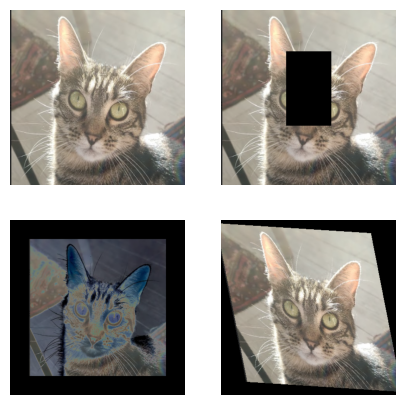
其他变换#
还有许多其他变换方式。例如:
删除图像的一部分;
在图像周围添加 填充(
padding);对图像进行 曝光(
solarize);应用精确的 仿射变换(
affine transformation)。
erase=T.Compose([T.RandomErasing(p=1)])
image_erase=erase(image)
solar=T.Compose([T.Pad(50),T.RandomSolarize(0.5,p=1)])
image_solar=solar(image)

affin=T.Compose([T.RandomAffine(degrees=30,scale=(0.8,1.2),shear=30)])
image_affin=affin(image)

plt.figure(figsize=(5,5))
plt.subplot(221)
plt.imshow(image.permute(1,2,0))
plt.axis("off")
plt.subplot(222)
plt.imshow(image_erase.permute(1,2,0))
plt.axis("off")
plt.subplot(223)
plt.imshow(image_solar.permute(1,2,0))
plt.axis("off")
plt.subplot(224)
plt.imshow(image_affin.permute(1,2,0))
plt.axis("off")
plt.show()
Clipping input data to the valid range for imshow with RGB data ([0..1] for floats or [0..255] for integers).
Clipping input data to the valid range for imshow with RGB data ([0..1] for floats or [0..255] for integers).
Clipping input data to the valid range for imshow with RGB data ([0..1] for floats or [0..255] for integers).
Clipping input data to the valid range for imshow with RGB data ([0..1] for floats or [0..255] for integers).
数据增强是一种非常有用的技术,可人工增加训练数据量,从而训练更大的模型而不发生 过拟合(overfitting)。在实践中,通常建议在神经网络训练中使用数据增强,但需谨慎选择方法。
建议您在数据集的部分样本上测试数据增强效果,以确保结果符合预期。
注:还有其他数据增强方法,例如在图像中添加噪声。更多可用变换请参阅 PyTorch 文档。
文本数据增强#
在 NLP 中也可以进行数据增强。以下是一些常用方法:
随机改变句子中某些词的位置(可提高模型鲁棒性,但需谨慎操作);
用同义词替换句子中的某些词;
对句子进行改写;
随机添加或删除句子中的词。
这些技术并非适用于所有 NLP 任务,使用时需格外小心。
注:随着大型语言模型(LLM)的兴起,即使数据量很少,也能通过 微调(fine-tuning)有效训练模型,从而减少了 NLP 中对数据增强的依赖。
音频数据增强#
在音频领域,数据增强也非常有用。以下是一些常用的音频数据增强技术:
添加噪声(高斯噪声或随机噪声),以提高模型在复杂环境下的性能;
对音频录音进行时间平移;
改变音频的播放速度;
调整音高(更高或更低)。