PyTorch 简介#
本笔记本将从 PyTorch 入门开始,PyTorch 是深度学习领域中非常流行的库。 我们将重新实现上一个笔记本中的神经网络,并使用 PyTorch 进行构建。
import random
import numpy as np
import matplotlib.pyplot as plt

# Import classiques des utilisateurs de pytorch
import torch
import torch.nn as nn
import torch.nn.functional as F
数据集与数据加载器#
我们将以类似上一个笔记本的方式重新构建数据集。此外,需要将输入特征 X 和标签 y 转换为张量(类似于 micrograd 中的 Value)。
# Initialisation du dataset
from sklearn.datasets import make_moons
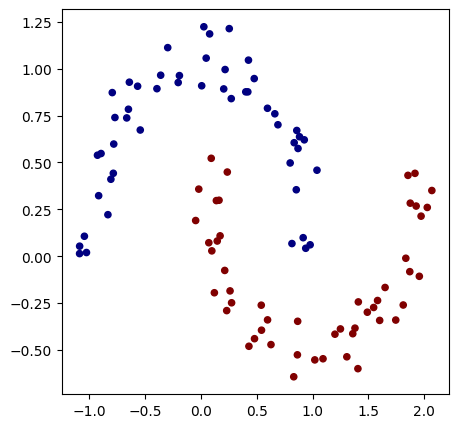
X, y = make_moons(n_samples=100, noise=0.1)
X=torch.tensor(X).float() # Conversion en tensor pytorch (équivalent de Value)
y=torch.tensor(y).float() # Conversion en tensor pytorch
y = y*2 - 1
plt.figure(figsize=(5,5))
plt.scatter(X[:,0], X[:,1], c=y, s=20, cmap='jet')
<matplotlib.collections.PathCollection at 0x7c6677d37350>
现在,我们将使用 PyTorch 的功能来创建数据集和数据加载器。 数据集仅包含输入特征和标签,而数据加载器通过提供来自数据集的随机小批量数据(数据加载器是一个迭代器),简化了随机梯度下降的使用。
from torch.utils.data import TensorDataset, DataLoader
# Création d'un dataset qui stocke les couples de valeurs X,y
dataset = TensorDataset(X, y)

# Création d'un dataloader qui permet de gérer automatiquement les mini-batchs pour la descente de gradient stochastique.
dataloader = DataLoader(dataset, batch_size=32, shuffle=True)
如需了解更多关于数据集和数据加载器的信息,可查阅 PyTorch 官方文档。
模型构建#
现在,我们构建一个包含 2 个隐藏层 的模型。
为此,我们将创建一个继承自 nn.Module 的 MLP 类。
然后,我们使用 nn.Linear(in_features, out_features)函数构建网络的各层,
该函数会创建一个全连接层,其输入维度为 in_features,输出维度为 out_features。
这一层由 out_features 个神经元组成,每个神经元与 in_features 个输入相连。
class mlp(nn.Module):
  def __init__(self, *args, **kwargs) -> None:
    super().__init__(*args, **kwargs)
    self.fc1=nn.Linear(2,16) # première couche cachée
    self.fc2=nn.Linear(16,16) # seconde couche cachée
    self.fc3=nn.Linear(16,1) # couche de sortie

  # La fonction forward est la fonction appelée lorsqu'on fait model(x)
  def forward(self,x):
    x=F.relu(self.fc1(x)) # le F.relu permet d'appliquer la fonction d'activation ReLU sur la sortie de notre couche
    x=F.relu(self.fc2(x))
    output=self.fc3(x)
    return output
model = mlp() # Couches d'entrée de taille 2, deux couches cachées de 16 neurones et un neurone de sortie
print(model)
print("Nombre de paramètres", sum(p.numel() for p in model.parameters()))
mlp(
  (fc1): Linear(in_features=2, out_features=16, bias=True)
  (fc2): Linear(in_features=16, out_features=16, bias=True)
  (fc3): Linear(in_features=16, out_features=1, bias=True)
)
Nombre de paramètres 337
该模型的参数数量与之前使用 micrograd 时的模型一致。
损失函数#
PyTorch 已经内置了一些常用的损失函数。在实现自定义损失函数之前,请先检查是否已存在。
这里,我们将使用 PyTorch 的 torch.nn.MSELoss 函数,其定义为:
\(MSE(y, \hat{y}) = \frac{1}{n} \sum_{i=1}^{n} (y_i - \hat{y}_i)^2\)
其中,\(y_i\) 是真实值(标签),\(\hat{y}_i\) 是预测值,\(n\) 是小批量数据中的样本总数。
在 PyTorch 中,该损失函数的实现非常简便:
criterion=torch.nn.MSELoss()
模型训练#
在训练过程中,我们需要定义 超参数 和 优化器。 优化器 是 PyTorch 中的一个类,用于指定训练过程中权重的更新方法(包括模型权重更新和学习率设置)。 常见的优化器包括:SGD、Adam、Adagrad、RMSProp 等。 这里我们使用 SGD(随机梯度下降)以复现上一个笔记本的训练条件,但在实际应用中,通常更推荐使用 Adam(自适应矩估计)。 如需了解优化器的更多细节及其差异,可参考优化器的加餐课程、PyTorch 官方文档 或 此博客文章。
# Hyper-paramètres
epochs = 100 # Nombre de fois où l'on parcoure l'ensemble des données d'entraînement
learning_rate=0.1
optimizer=torch.optim.SGD(model.parameters(),lr=learning_rate)
/home/aquilae/anaconda3/envs/dev/lib/python3.11/site-packages/tqdm/auto.py:21: TqdmWarning: IProgress not found. Please update jupyter and ipywidgets. See https://ipywidgets.readthedocs.io/en/stable/user_install.html
  from .autonotebook import tqdm as notebook_tqdm
我们还可以使用 学习率调度器(scheduler),在训练过程中动态调整学习率,以加速模型收敛(例如,从较高的学习率开始,逐渐降低)。 为了实现训练过程中学习率逐渐减小(如 micrograd 示例中所示),可以使用 LinearLR。 如需了解不同类型的调度器,可查阅 PyTorch 官方文档。
scheduler=torch.optim.lr_scheduler.LinearLR(optimizer=optimizer,start_factor=1,end_factor=0.05)
for i in range(epochs):
  loss_epoch=0
  accuracy=[]
  for batch_X, batch_y in dataloader:
    scores=model(batch_X)
    loss=criterion(scores,batch_y.unsqueeze(1))
    optimizer.zero_grad()
    loss.backward()
    optimizer.step()
    #scheduler.step() # Pour activer le scheduler
    loss_epoch+=loss

    accuracy += [(label > 0) == (scorei.data > 0) for label, scorei in zip(batch_y, scores)]
  accuracy=sum(accuracy) / len(accuracy)

  if i % 10 == 0:
    print(f"step {i} loss {loss_epoch}, précision {accuracy*100}%")
step 0 loss 0.12318143993616104, précision tensor([100.])%
step 10 loss 0.1347985863685608, précision tensor([100.])%
step 20 loss 0.10458286106586456, précision tensor([100.])%
step 30 loss 0.14222581684589386, précision tensor([100.])%
step 40 loss 0.1081438660621643, précision tensor([100.])%
step 50 loss 0.10838648676872253, précision tensor([100.])%
step 60 loss 0.09485019743442535, précision tensor([100.])%
step 70 loss 0.07788567245006561, précision tensor([100.])%
step 80 loss 0.10796503722667694, précision tensor([100.])%
step 90 loss 0.07869727909564972, précision tensor([100.])%
训练速度明显更快!
我们可以将训练结果可视化:
h = 0.25
x_min, x_max = X[:, 0].min() - 1, X[:, 0].max() + 1
y_min, y_max = X[:, 1].min() - 1, X[:, 1].max() + 1
xx, yy = np.meshgrid(np.arange(x_min, x_max, h),
                     np.arange(y_min, y_max, h))
Xmesh = np.c_[xx.ravel(), yy.ravel()]

inputs=torch.tensor(Xmesh).float()
scores=model(inputs)

Z = np.array([s.data > 0 for s in scores])
Z = Z.reshape(xx.shape)

fig = plt.figure()
plt.contourf(xx, yy, Z, cmap=plt.cm.Spectral, alpha=0.8)
plt.scatter(X[:, 0], X[:, 1], c=y, s=40, cmap=plt.cm.Spectral)
plt.xlim(xx.min(), xx.max())
plt.ylim(yy.min(), yy.max())
(-1.6418534517288208, 2.108146548271179)
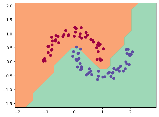
如图所示,训练过程顺利进行,并且模型对数据的分类效果良好。