激活函数与初始化

在本课程中，我们将回顾第5课中介绍的全连接模型（Fully Connected）。我们将研究网络初始化时，激活函数在整个网络中的表现行为。本课程灵感来源于 Andrej Karpathy 的课程《Building makemore Part 3: 激活函数、梯度与批归一化》。

神经网络具有以下优点：

• 灵活性高：能够解决多种问题。

• 实现简单：框架易于构建。

但优化过程复杂，特别是在深度网络中，调试与参数调整往往面临挑战。

代码回顾

我们将重用第5课《NLP》中笔记本3：全连接网络的代码。

import torch
import torch.nn.functional as F
import matplotlib.pyplot as plt
%matplotlib inline

words = open('../05_NLP/prenoms.txt', 'r').read().splitlines()
chars = sorted(list(set(''.join(words))))
stoi = {s:i+1 for i,s in enumerate(chars)}
stoi['.'] = 0
itos = {i:s for s,i in stoi.items()}

出于教学目的，我们不使用 PyTorch 的数据集与数据加载器。我们将在训练开始时，通过第一个**批次（batch）**计算损失值（loss）。整体逻辑不变，唯一区别是：

• 每次迭代随机抽取一个批次，而非每轮遍历整个数据集。

block_size = 3 # Contexte

def build_dataset(words):  
  X, Y = [], []
  
  for w in words:
    context = [0] * block_size
    for ch in w + '.':
      ix = stoi[ch]
      X.append(context)
      Y.append(ix)
      context = context[1:] + [ix] 

  X = torch.tensor(X)
  Y = torch.tensor(Y)
  print(X.shape, Y.shape)
  return X, Y

import random
random.seed(42)
random.shuffle(words)
n1 = int(0.8*len(words))
n2 = int(0.9*len(words))

Xtr,  Ytr  = build_dataset(words[:n1])     # 80%
Xdev, Ydev = build_dataset(words[n1:n2])   # 10%
Xte,  Yte  = build_dataset(words[n2:])     # 10%

torch.Size([180834, 3]) torch.Size([180834])
torch.Size([22852, 3]) torch.Size([22852])
torch.Size([22639, 3]) torch.Size([22639])

embed_dim=10 # Dimension de l'embedding de C
hidden_dim=200 # Dimension de la couche cachée

C = torch.randn((46, embed_dim))
W1 = torch.randn((block_size*embed_dim, hidden_dim))
b1 = torch.randn(hidden_dim)
W2 = torch.randn((hidden_dim, 46))
b2 = torch.randn(46)
parameters = [C, W1, b1, W2, b2]
for p in parameters:
  p.requires_grad = True

max_steps = 200000
batch_size = 32
lossi = []

for i in range(max_steps):
  # Permet de construire un mini-batch
  ix = torch.randint(0, Xtr.shape[0], (batch_size,))
  
  # Forward
  Xb, Yb = Xtr[ix], Ytr[ix] 
  emb = C[Xb] 
  embcat = emb.view(emb.shape[0], -1)
  hpreact = embcat @ W1 + b1 

  h = torch.tanh(hpreact) 
  logits = h @ W2 + b2 
  loss = F.cross_entropy(logits, Yb)
  
  # Retropropagation
  for p in parameters:
    p.grad = None
  
  loss.backward()
  # Mise à jour des paramètres
  lr = 0.1 if i < 100000 else 0.01 # On descend le learning rate d'un facteur 10 après 100000 itérations
  for p in parameters:
    p.data += -lr * p.grad

  if i % 10000 == 0:
    print(f'{i:7d}/{max_steps:7d}: {loss.item():.4f}')
  lossi.append(loss.log10().item())

      0/ 200000: 21.9772
  10000/ 200000: 2.9991
  20000/ 200000: 2.5258
  30000/ 200000: 1.9657
  40000/ 200000: 2.4326
  50000/ 200000: 1.7670
  60000/ 200000: 2.1324
  70000/ 200000: 2.4160
  80000/ 200000: 2.2237
  90000/ 200000: 2.3905
 100000/ 200000: 1.9304
 110000/ 200000: 2.1710
 120000/ 200000: 2.3444
 130000/ 200000: 2.0970
 140000/ 200000: 1.8623
 150000/ 200000: 1.9792
 160000/ 200000: 2.4602
 170000/ 200000: 2.0968
 180000/ 200000: 2.0466
 190000/ 200000: 2.3746

plt.plot(lossi)

[<matplotlib.lines.Line2D at 0x7f028467b990>]

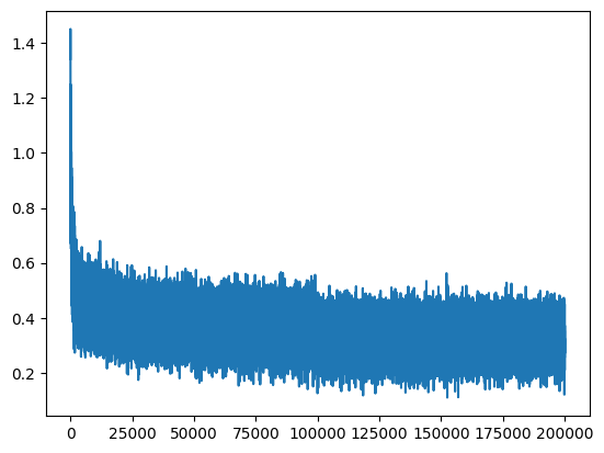
由于每次计算损失值时使用的小批次数据相对于整个训练集规模较小，结果会存在较大波动（噪声）。

初始化时损失值异常偏高

训练过程总体正常，但初始阶段的损失值异常偏高。理论上，若每个字母出现的概率均等（即 \(P=\frac{1}{46}\)），则初始损失值应接近该分布的负对数似然： $\(-ln\left(\frac{1}{46}\right) = 3.83\)$ 因此，首次计算的损失值应与该数量级相当。

问题示例分析

为理解该问题，我们通过一个小示例观察初始化方式对损失值的影响。假设logits中所有权重初始化为0，此时输出概率将均匀分布。

logits=torch.tensor([0.0,0.0,0.0,0.0])
probs=torch.softmax(logits,dim=0)
loss= -probs[1].log()
probs,loss

(tensor([0.2500, 0.2500, 0.2500, 0.2500]), tensor(1.3863))

然而，将神经网络权重初始化为0并非最佳实践。我们采用标准正态分布（均值为0，方差为1）进行随机初始化。

logits=torch.randn(4)
probs=torch.softmax(logits,dim=0)
loss= -probs[1].log()
probs,loss

(tensor([0.3143, 0.0607, 0.3071, 0.3178]), tensor(2.8012))

问题显而易见：正态分布的随机性导致logits向某一侧倾斜（可多次运行上述代码验证）。解决方案：

• 将logits向量乘以一个小系数（如0.01），以降低初始权重值，使softmax输出更均匀。

logits=torch.randn(4)*0.01
probs=torch.softmax(logits,dim=0)
loss= -probs[1].log()
probs,loss

(tensor([0.2489, 0.2523, 0.2495, 0.2493]), tensor(1.3772))

经过调整后，损失值接近均匀概率分布的理论值。

注意：偏置项（bias）可初始化为0，因为初始阶段正/负偏置缺乏实际意义。

使用调整后初始化的训练

我们重用之前的代码，但采用新的初始化参数。

C = torch.randn((46, embed_dim))
W1 = torch.randn((block_size*embed_dim, hidden_dim))*0.01 # On initialise les poids à une petite valeur
b1 = torch.randn(hidden_dim) *0 # On initialise les biais à 0
W2 = torch.randn((hidden_dim, 46))*0.01
b2 = torch.randn(46)*0 
parameters = [C, W1, b1, W2, b2]
for p in parameters:
  p.requires_grad = True

lossi = []

for i in range(max_steps):
  ix = torch.randint(0, Xtr.shape[0], (batch_size,))
  Xb, Yb = Xtr[ix], Ytr[ix] 
  emb = C[Xb] 
  embcat = emb.view(emb.shape[0], -1)
  hpreact = embcat @ W1 + b1 
  h = torch.tanh(hpreact) 
  logits = h @ W2 + b2 
  loss = F.cross_entropy(logits, Yb)
  
  for p in parameters:
    p.grad = None
  loss.backward()
  lr = 0.1 if i < 100000 else 0.01 
  for p in parameters:
    p.data += -lr * p.grad
  if i % 10000 == 0:
    print(f'{i:7d}/{max_steps:7d}: {loss.item():.4f}')
  lossi.append(loss.log10().item())

      0/ 200000: 3.8304
  10000/ 200000: 2.4283
  20000/ 200000: 2.0651
  30000/ 200000: 2.1124
  40000/ 200000: 2.3158
  50000/ 200000: 2.2752
  60000/ 200000: 2.1887
  70000/ 200000: 2.1783
  80000/ 200000: 1.8120
  90000/ 200000: 2.3178
 100000/ 200000: 2.0973
 110000/ 200000: 1.8992
 120000/ 200000: 1.6917
 130000/ 200000: 2.2747
 140000/ 200000: 1.8054
 150000/ 200000: 2.3569
 160000/ 200000: 2.4231
 170000/ 200000: 2.0711
 180000/ 200000: 2.1379
 190000/ 200000: 1.8419

plt.plot(lossi)

[<matplotlib.lines.Line2D at 0x7f0278310110>]

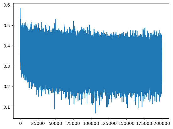
现在，损失曲线不再从异常高值开始，这加速了模型的优化过程。

另一个问题

虽然高损失值似乎并非致命问题，但不当的权重初始化会引发其他隐患。我们以未缩放初始化（即未乘以0.01系数）的首轮训练为例进行分析。

C = torch.randn((46, embed_dim))
W1 = torch.randn((block_size*embed_dim, hidden_dim)) 
b1 = torch.randn(hidden_dim) 
W2 = torch.randn((hidden_dim, 46))
b2 = torch.randn(46)
parameters = [C, W1, b1, W2, b2]
for p in parameters:
  p.requires_grad = True

ix = torch.randint(0, Xtr.shape[0], (batch_size,))
Xb, Yb = Xtr[ix], Ytr[ix] 
emb = C[Xb] 
embcat = emb.view(emb.shape[0], -1)
hpreact = embcat @ W1 + b1 
h = torch.tanh(hpreact) 
logits = h @ W2 + b2 
loss = F.cross_entropy(logits, Yb)
  
for p in parameters:
  p.grad = None
loss.backward()

我们观察激活函数 tanh输出值的直方图分布。

plt.hist(h.view(-1).tolist(),50);

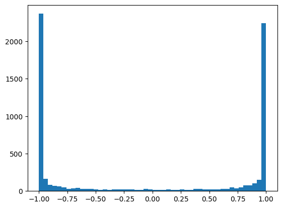
观察发现，大多数值聚集在1或-1附近。

问题所在： 根据链式法则，梯度计算需逐层相乘。tanh函数的导数为： $\(tanh'(t) = 1 - t^2\)\( 当 \)t$ 接近1或-1时，导数趋近于0（渐近线），导致梯度消失。这意味着：

• 初始阶段梯度无法有效传播，优化过程受阻。

我们可视化每个神经元的激活值以进一步分析。

plt.figure(figsize=(20,10))
plt.imshow(h.abs()>0.99,cmap='gray',interpolation='nearest')

<matplotlib.image.AxesImage at 0x7f02780ae550>

图中白色点代表梯度近似为0的神经元。

“死神经元”：

• 若某列全部为白色，说明该神经元在整个批次中均未激活，成为“死神经元”，对结果无贡献且无法优化。

补充说明：

• 该问题并非tanh独有：sigmoid与ReLU同样可能受此影响。

• 由于本示例模型较小，问题影响有限；但在深度网络中，此类问题会严重阻碍训练，需定期检查各层激活值。

• 死神经元可能出现在初始化阶段，或因学习率过高等原因在训练过程中产生。

如何解决该问题？

幸运的是，该问题的解决方案与高损失值问题相同。我们验证使用新初始化参数后，激活值分布与死神经元情况。

C = torch.randn((46, embed_dim))
W1 = torch.randn((block_size*embed_dim, hidden_dim)) *0.01# On initialise les poids à une petite valeur
b1 = torch.randn(hidden_dim) *0 # On initialise les biais à 0
W2 = torch.randn((hidden_dim, 46)) *0.01
b2 = torch.randn(46)*0 
parameters = [C, W1, b1, W2, b2]
for p in parameters:
  p.requires_grad = True

ix = torch.randint(0, Xtr.shape[0], (batch_size,))
Xb, Yb = Xtr[ix], Ytr[ix] 
emb = C[Xb] 
embcat = emb.view(emb.shape[0], -1)
hpreact = embcat @ W1 + b1 
h = torch.tanh(hpreact) 
logits = h @ W2 + b2 
loss = F.cross_entropy(logits, Yb)
  
for p in parameters:
  p.grad = None
loss.backward()

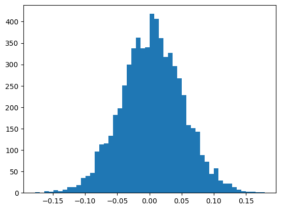
plt.hist(h.view(-1).tolist(),50);

plt.figure(figsize=(20,10))
plt.imshow(h.abs()>0.99,cmap='gray',interpolation='nearest')

<matplotlib.image.AxesImage at 0x7f025c538190>

现在一切正常！

初始化的最优参数

由于该问题极为关键，相关研究层出不穷。其中里程碑式论文《Delving Deep into Rectifiers》提出了Kaiming初始化方法，为不同激活函数提供了保证网络整体分布均衡的初始化参数。

该方法已集成至PyTorch，后续创建的PyTorch层将默认采用此初始化策略。

为何将如此重要的内容放入“附录”？

该问题确实至关重要，但使用PyTorch时，框架已内置正确的初始化方案，通常无需手动调整。

此外，已有多种方法缓解该问题，如：

• 批归一化（Batch Norm）：在下一笔记本中将详细介绍，通过标准化激活前的值改善梯度传播。

• 残差连接（Residual Connections）：确保梯度能跨层传播，不受激活函数影响过大。

虽然理解这些原理有助于深入优化，但在实际应用中，PyTorch等框架的默认设置已足够支持大多数训练任务。