生成对抗网络(GAN)的实现#
现在我们将实现一个 GAN。为此,我们将参考论文《基于深度卷积生成对抗网络的无监督表示学习》,以生成类似 MNIST 数据集中数字“5”的图像。
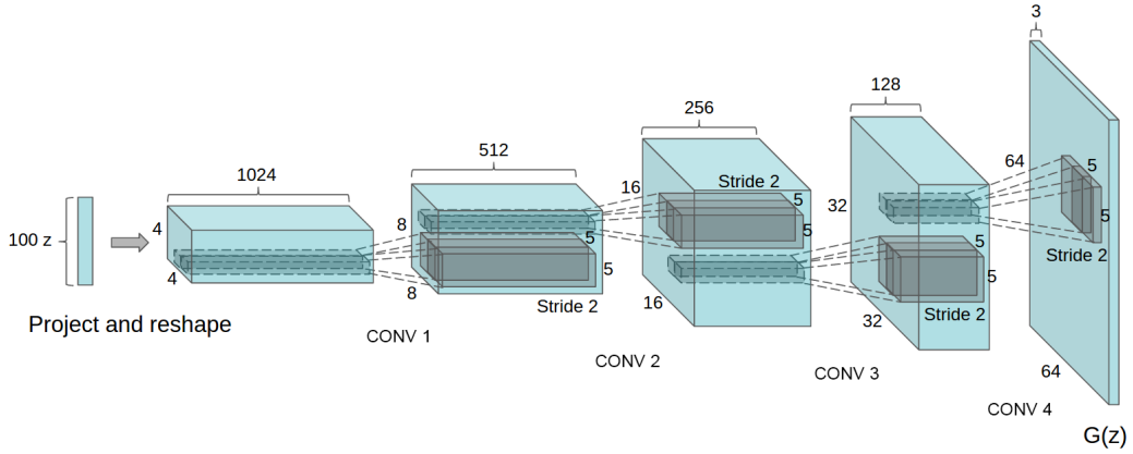
上图为 DCGAN 生成器的架构示意图。
import torch
import torch.nn as nn
import torch.nn.functional as F
import numpy as np
import matplotlib.pyplot as plt
import torchvision.datasets as datasets
import torchvision.transforms as transforms
from torch.utils.data import DataLoader,Subset
import random
/home/aquilae/anaconda3/envs/dev/lib/python3.11/site-packages/tqdm/auto.py:21: TqdmWarning: IProgress not found. Please update jupyter and ipywidgets. See https://ipywidgets.readthedocs.io/en/stable/user_install.html
  from .autonotebook import tqdm as notebook_tqdm
数据集#
首先,我们加载 MNIST 数据集:
transform=transforms.Compose([
    transforms.ToTensor(),
    transforms.Resize((32,32)),
])
train_data = datasets.MNIST(root='./../data', train=True, transform=transform, download=True)
test_data = datasets.MNIST(root='./../data', train=False, transform=transform, download=True)


indices = [i for i, label in enumerate(train_data.targets) if label == 5]
# On créer un nouveau dataset avec uniquement les 5
train_data = Subset(train_data, indices)

# all_indices = list(range(len(train_data)))
# random.shuffle(all_indices)
# selected_indices = all_indices[:5000]
# train_data = Subset(train_data, selected_indices)


print("taille du dataset d'entrainement : ",len(train_data))
print("taille d'une image : ",train_data[0][0].numpy().shape)

train_loader = DataLoader(dataset=train_data, batch_size=64, shuffle=True)
test_loader = DataLoader(dataset=test_data, batch_size=64, shuffle=False)
taille du dataset d'entrainement :  5421
taille d'une image :  (1, 32, 32)
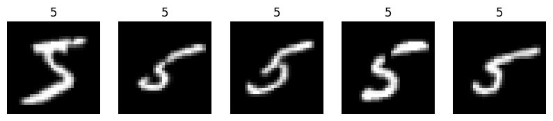
# Visualisons quelques images
plt.figure(figsize=(10, 10))
for i in range(5):
  plt.subplot(1, 5, i+1)
  plt.imshow(train_data[i][0].squeeze(), cmap='gray')
  plt.axis('off')
  plt.title(train_data[i][1])
构建模型#
现在我们可以实现这两个模型。首先,我们来看论文中描述的架构细节。
基于论文中的信息(见 notebook 上方的图示),我们可以构建生成器模型。由于我们处理的是 \(28 \times 28\) 大小的图像(而非论文中的 \(64 \times 64\)),因此架构会相应简化。
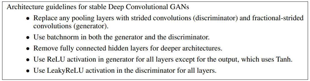
注意:论文中提到的 fractional-strided convolutions(分数步长卷积)实际上是指转置卷积,而 fractional-strided convolutions 这一术语现今已不再常用。
def convT_bn_relu(in_channels, out_channels, kernel_size, stride, padding):
  return nn.Sequential(
    nn.ConvTranspose2d(in_channels, out_channels, kernel_size, stride, padding,bias=False),
    nn.BatchNorm2d(out_channels),
    nn.ReLU()
  )

class generator(nn.Module):
  def __init__(self, z_dim=100,features_g=64):
    super(generator, self).__init__()
    self.gen = nn.Sequential(
      convT_bn_relu(z_dim, features_g*8, kernel_size=4, stride=1, padding=0),
      convT_bn_relu(features_g*8, features_g*4, kernel_size=4, stride=2, padding=1),
      convT_bn_relu(features_g*4, features_g*2, kernel_size=4, stride=2, padding=1),
      nn.ConvTranspose2d(features_g*2, 1, kernel_size=4, stride=2, padding=1),
      nn.Tanh()
    )
  def forward(self, x):
    return self.gen(x)

z= torch.randn(64,100,1,1)
gen = generator()
img = gen(z)
print(img.shape)
torch.Size([64, 1, 32, 32])
论文没有直接描述判别器的架构。我们将采用与生成器相反方向的类似架构来构建判别器。
def conv_bn_lrelu(in_channels, out_channels, kernel_size, stride, padding):
  return nn.Sequential(
    nn.Conv2d(in_channels, out_channels, kernel_size, stride, padding,bias=False),
    nn.BatchNorm2d(out_channels),
    nn.LeakyReLU()
  )

class discriminator(nn.Module):
  def __init__(self, features_d=64) -> None:
    super().__init__()
    self.discr = nn.Sequential(
      conv_bn_lrelu(1, features_d, kernel_size=3, stride=2, padding=1),
      conv_bn_lrelu(features_d, features_d*2, kernel_size=3, stride=2, padding=1),
      conv_bn_lrelu(features_d*2, features_d*4, kernel_size=3, stride=2, padding=1),
      nn.Conv2d(256, 1, kernel_size=3, stride=2, padding=0),
      nn.Sigmoid()
    )

  def forward(self, x):
    return self.discr(x)
dummy = torch.randn(64,1,32,32)
disc = discriminator()
out = disc(dummy)
print(out.shape)
torch.Size([64, 1, 1, 1])
模型训练#
现在进入核心环节。GAN 的训练循环比我们之前见过的模型训练循环要复杂得多。 首先,我们定义训练超参数并初始化模型:
epochs = 50
lr=0.001
z_dim = 100
features_d = 64
features_g = 64

device = torch.device('cuda' if torch.cuda.is_available() else 'cpu')
gen = generator(z_dim, features_g).to(device)
disc = discriminator(features_d).to(device)

opt_gen = torch.optim.Adam(gen.parameters(), lr=lr)
opt_disc = torch.optim.Adam(disc.parameters(), lr=lr*0.05)
criterion = nn.BCELoss()
我们还将创建一个固定噪声 fixed_noise,以便在每个训练步骤中可视化模型的生成效果。
fixed_noise = torch.randn(64, z_dim, 1, 1, device=device)
在构建训练循环前,我们总结以下关键步骤:
从训练数据集中获取 batch_size 个样本,并用判别器预测其标签;
用生成器生成 batch_size 个样本,并预测其标签;
基于上述两组损失更新判别器的权重;
由于判别器已更新,重新预测生成数据的标签;
基于这些预测值计算损失,并更新生成器。
all_fake_images = []
for epoch in range(epochs):
  lossD_epoch = 0
  lossG_epoch = 0
  for real_images,_ in train_loader:
    real_images=real_images.to(device)
    pred_real = disc(real_images).view(-1)
    lossD_real = criterion(pred_real, torch.ones_like(pred_real)) # Les labels sont 1 pour les vraies images

    batch_size = real_images.shape[0]
    input_noise = torch.randn(batch_size, z_dim, 1, 1, device=device)
    fake_images = gen(input_noise)
    pred_fake = disc(fake_images.detach()).view(-1)
    lossD_fake = criterion(pred_fake, torch.zeros_like(pred_fake)) # Les labels sont 0 pour les fausses images

    lossD=lossD_real + lossD_fake
    lossD_epoch += lossD.item()
    disc.zero_grad()
    lossD.backward()
    opt_disc.step()

    # On refait l'inférence pour les images générées (avec le discriminateur mis à jour)
    pred_fake = disc(fake_images).view(-1)
    lossG=criterion(pred_fake, torch.ones_like(pred_fake)) # On veut que le générateur trompe le discriminateur donc on veut que les labels soient 1
    lossG_epoch += lossG.item()
    gen.zero_grad()
    lossG.backward()
    opt_gen.step()

  # On génère des images avec le générateur
  if epoch % 10 == 0 or epoch==0:
    print(f"Epoch [{epoch}/{epochs}] Loss D: {lossD_epoch/len(train_loader):.4f}, loss G: {lossG_epoch/len(train_loader):.4f}")
    gen.eval()
    fake_images = gen(fixed_noise)
    all_fake_images.append(fake_images)
    #cv2.imwrite(f"gen/image_base_gan_{epoch}.png", fake_images[0].squeeze().detach().cpu().numpy()*255.0)
    gen.train()
/home/aquilae/anaconda3/envs/dev/lib/python3.11/site-packages/torch/nn/modules/conv.py:952: UserWarning: Plan failed with a cudnnException: CUDNN_BACKEND_EXECUTION_PLAN_DESCRIPTOR: cudnnFinalize Descriptor Failed cudnn_status: CUDNN_STATUS_NOT_SUPPORTED (Triggered internally at ../aten/src/ATen/native/cudnn/Conv_v8.cpp:919.)
  return F.conv_transpose2d(
Epoch [0/50] Loss D: 0.4726, loss G: 2.0295
Epoch [10/50] Loss D: 0.1126, loss G: 3.6336
Epoch [20/50] Loss D: 0.0767, loss G: 4.0642
Epoch [30/50] Loss D: 0.0571, loss G: 4.5766
Epoch [40/50] Loss D: 0.0178, loss G: 5.3689
可视化训练过程中生成的图像。
index=0
image_begin = all_fake_images[0][index]
image_mid = all_fake_images[len(all_fake_images)//2][index]
image_end = all_fake_images[-1][index]

# Création de la figure
plt.figure(figsize=(10, 5))

# Affichage de l'image du début de l'entraînement
plt.subplot(1, 3, 1)
plt.imshow(image_begin.squeeze().detach().cpu().numpy(), cmap='gray')
plt.axis('off')
plt.title("Début de l'entrainement")

# Affichage de l'image du milieu de l'entraînement
plt.subplot(1, 3, 2)
plt.imshow(image_mid.squeeze().detach().cpu().numpy(), cmap='gray')
plt.axis('off')
plt.title("Milieu de l'entrainement")

# Affichage de l'image de la fin de l'entraînement
plt.subplot(1, 3, 3)
plt.imshow(image_end.squeeze().detach().cpu().numpy(), cmap='gray')
plt.axis('off')
plt.title("Fin de l'entrainement")

# Affichage de la figure
plt.tight_layout()
plt.show()
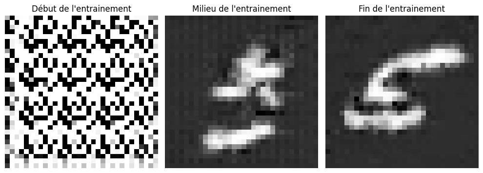
可以看到,我们的生成器现在能生成类似数字“5”的模糊图像。 如果你有兴趣深入,可以尝试改进模型,并在整个 MNIST 数据集(所有数字)上训练。 另一个有益的练习是实现一个条件 GAN(Conditional GAN)。