使用 Transformer 的计算机视觉#
在本教程中,我们将使用 Hugging Face 的 Transformers 库处理图像。为了避免笔记本过载,部分函数已存放在 utils/util.py 中。
零样本对象检测(Zero-Shot)#
图像中的对象检测是计算机视觉中的一项核心任务。零样本模型非常实用,因为它们无需微调即可检测任意对象。只需提供一张图像和包含要检测类别的文本提示即可。
实现步骤#
我们选择了谷歌的 OWL-ViT 模型(google/owlvit-base-patch32),因为它轻量且适用于大多数设备。我们将使用 Hugging Face 的 pipeline 进行实现:
from transformers import pipeline
from PIL import Image
import cv2
import numpy as np
import matplotlib.pyplot as plt

zeroshot = pipeline("zero-shot-object-detection", model="google/owlvit-base-patch32")
/home/aquilae/anaconda3/envs/dev/lib/python3.11/site-packages/tqdm/auto.py:21: TqdmWarning: IProgress not found. Please update jupyter and ipywidgets. See https://ipywidgets.readthedocs.io/en/stable/user_install.html
  from .autonotebook import tqdm as notebook_tqdm
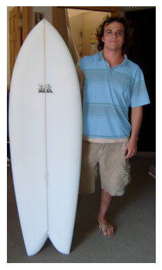
首先,我们来看一下待处理的图像。
image=Image.open("images/coco.jpg") # Image extraite de la base de données COCO (https://cocodataset.org/#home)

plt.imshow(image)
plt.axis('off')
plt.show()
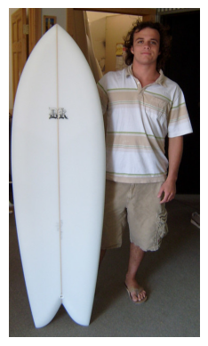
接下来,我们将使用模型绘制预测的检测框。
from utils.util import draw_box

text_prompt = "surfboard" # Vous pouvez changer la classe pour détecter autre chose "person" ou "surfboard"
output = zeroshot(image,candidate_labels = [text_prompt])
cv_image=draw_box(image,output)

plt.imshow(cv_image)
plt.axis('off')
plt.show()

现在,您已经学会如何用几行代码实现一个零样本对象检测器了。
图像描述生成#
图像描述生成是指为图像自动生成文本描述。模型接收图像作为输入,并输出对应的描述文本。
实现步骤#
同样,我们使用 Hugging Face 的 pipeline。此处采用 Salesforce 的 BLIP 模型(Salesforce/blip-image-captioning-base)。
captionner = pipeline("image-to-text", model="Salesforce/blip-image-captioning-base")
我们将使用同一张图像生成描述。
result=captionner(image)
print(result[0]['generated_text'])
a man holding a surfboard in a room
模型生成的描述为“一个男子在房间里拿着冲浪板”,这与图像内容相符。 现在,您已经学会如何生成图像描述。这在自动创建数据集时非常有用。
零样本图像分类(Zero-Shot)#
除了零样本对象检测,我们还可以进行零样本图像分类。原理类似,但这次我们需要提供至少两个文本描述,模型将给出图像分别对应每个描述的概率。
实现步骤#
我们将使用一张我的猫的照片来判断它的品种:
image=Image.open("images/tigrou.png") # Image extraite de la base de données COCO (https://cocodataset.org/#home)

plt.imshow(image)
plt.axis('off')
plt.show()

我们将测试模型是否能判断它是缅因猫还是欧洲短毛猫。
我们将使用 OpenAI 的 CLIP 模型(openai/clip-vit-base-patch32)。为了展示多样性,此处我们将直接调用 Hugging Face 库的其他函数,而非使用 pipeline。
from transformers import AutoProcessor, AutoModelForZeroShotImageClassification

processor = AutoProcessor.from_pretrained("openai/clip-vit-base-patch32")
model = AutoModelForZeroShotImageClassification.from_pretrained("openai/clip-vit-base-patch32")
/home/aquilae/anaconda3/envs/dev/lib/python3.11/site-packages/huggingface_hub/file_download.py:1132: FutureWarning: `resume_download` is deprecated and will be removed in version 1.0.0. Downloads always resume when possible. If you want to force a new download, use `force_download=True`.
  warnings.warn(
labels = ["a photo of a european shorthair", "a photo of maine coon"]
inputs = processor(text=labels,images=image,return_tensors="pt",padding=True)
outputs = model(**inputs)

# Transformation des outputs pour obtenir des probabilités
print("Probabilité de a photo of a european shorthair : ",outputs.logits_per_image.softmax(dim=1)[0][0].item())
print("Probabilité de a photo of maine coon : ",outputs.logits_per_image.softmax(dim=1)[0][1].item())
Probabilité de a photo of a european shorthair :  0.9104425311088562
Probabilité de a photo of maine coon :  0.08955750614404678
模型相当确信这是一只欧洲短毛猫,而实际上它判断正确。
图像分割#
在这个示例中,我们将使用 Meta 的 SAM 模型,它能够分割图像中的任意对象。
实现步骤#
sam = pipeline("mask-generation","Zigeng/SlimSAM-uniform-77")
image=Image.open("images/coco.jpg") # Image extraite de la base de données COCO (https://cocodataset.org/#home)

plt.imshow(image)
plt.axis('off')
plt.show()
# ATTENTION : le traitement peut prendre plusieurs minutes
output=sam(image, points_per_batch=32)
masks=output["masks"]
from utils.util import draw_masks
image_np=draw_masks(image,masks)

plt.imshow(image_np)
plt.axis('off')
plt.show()

如您所见,我们已经分割出了图像中的所有对象。不过,处理时间较长… 为了获得更合理的推理时间,我们可以使用图像中某一点的坐标提示。这能够指定处理区域并加快结果生成速度。 注意:Hugging Face 的 pipeline 不支持这一任务。
from transformers import SamModel, SamProcessor
model = SamModel.from_pretrained("Zigeng/SlimSAM-uniform-77")

processor = SamProcessor.from_pretrained("Zigeng/SlimSAM-uniform-77")
现在,我们创建坐标提示并可视化该点:
input_points = [[[300, 200]]]
image_np= np.array(image)
cv2.circle(image_np,input_points[0][0],radius=3,color=(255,0,0),thickness=5)
plt.imshow(image_np)
plt.axis('off')
plt.show()

inputs = processor(image,input_points=input_points,return_tensors="pt")
outputs = model(**inputs)
predicted_masks = processor.image_processor.post_process_masks(
  outputs.pred_masks,
  inputs["original_sizes"],
  inputs["reshaped_input_sizes"]
)
处理速度明显加快!
SAM 默认生成 3 个掩码。每个掩码代表一种可能的图像分割方式。您可以修改 mask_number 的值来查看不同的掩码。
mask_number=2 # 0,1 or 2
mask=predicted_masks[0][:, mask_number]
image_np=draw_masks(image,mask)
plt.imshow(image_np)
plt.axis('off')
plt.show()
在这个示例中,3 个掩码都很合理:
第 1 个掩码分割了整个人
第 2 个掩码分割了衣服
第 3 个掩码仅分割了 T 恤
您可以尝试更改坐标点,观察生成的不同掩码。
深度估计#
深度估计是计算机视觉中的一项关键任务。它在以下场景中非常有用:
自动驾驶:估计与前方车辆的距离
工业应用:根据剩余空间组织包裹中的物品
在这个示例中,我们使用 Intel 的 DPT 模型(Intel/dpt-hybrid-midas),它接收图像输入并输出深度图。
实现步骤#
depth_estimator = pipeline(task="depth-estimation",model="Intel/dpt-hybrid-midas")
image=Image.open("images/coco2.jpg") # Image extraite de la base de données COCO (https://cocodataset.org/#home)

plt.imshow(image)
plt.axis('off')
plt.show()

outputs = depth_estimator(image)
outputs["predicted_depth"].shape
torch.Size([1, 384, 384])
我们使用 PyTorch 将预测的深度图尺寸调整为与原始图像一致,然后生成深度图的可视化图像。
import torch
prediction = torch.nn.functional.interpolate(outputs["predicted_depth"].unsqueeze(1),size=image.size[::-1],
                                             mode="bicubic",align_corners=False)
output = prediction.squeeze().numpy()
formatted = (output * 255 / np.max(output)).astype("uint8")
depth = Image.fromarray(formatted)

fig, (ax1, ax2) = plt.subplots(1, 2, figsize=(12, 6))
ax1.imshow(image)
ax1.axis('off')
ax2.imshow(depth)
ax2.axis('off')
plt.show()

在深度图中,明亮的颜色代表距离更近的对象。可以清楚地看到:
道路(非常明亮)距离最近
公交车(较明亮)距离稍远
因此,该深度图的精度较高。